1
University of Bialystok
Faculty of Physics
Statics and Dynamics of Magnetization in:
Patterned Permalloy and Ion-Irradiated Co
and FeAl Nanostructures
Nadeem Tahir
Promotor: dr hab. Ryszard Gieniusz
2
Abstract
The understanding of magnetization reversal behavior and spin wave excitation spectrum in the micro- and nanometer length scale of ferromagnetic elements has attracted much attention in the recent years due to discoveries of fundamental new physics and their potential applications such as magneto-optical devices, magnetic recording media, and sensors. Especially interesting are patterned magnetic nanostructures, such as magnonic crystals (MCs), metamaterials where magnetic properties are modulated in periodic manners. In the this dissertation, three topics related to the modification of magnetic properties were distinguished: through patterning (removal of magnetic material) in permalloy (Py) and ion irradiation in Fe60Al40 and cobalt (Co) thin films. These samples were studied by combining
different experimental techniques such as magnetooptical Kerr effect microscopy (MOKE) and three spectrometries: Brillouin light scattering (BLS), X-band ferromagnetic resonance (FMR) and vector network analyzer ferromagnetic resonance (VNA-FMR). Initial chemically ordered B2-phase Fe60Al40 (paramagnetic) thin films was transformed to chemically
disordered A2-phase (ferromagnetic) by Ne+ ions-irradiations with varying energies in the range of 0-30 keV (keeping fluence constant 6 ×10¹⁴ ions cm-2). The relationship of effective thickness (defined by energy of ions) with different magnetization processes and evolution of magnetic domains were sorted out. Spin wave excitations at Damon-Eshbach (DE) and standing spin waves (SSW) modes were identified in relation to ferromagnetic layer thickness/(energies of the irradiated ions). Depth varying magnetization set the pinning mechanisms for spin waves which accounts additional mode across A2/B2-phase boundary. The analytical calculations were in good agreement with the experimental results where spin-wave modes were directly related to the effective ferromagnetic thickness. In 1D reprogrammable stripe patterned Fe60Al40 sample, the existence of binary re-programmable
magnetization configurations, demonstrated the possibility to apply disorder induced ferromagnetic structures for creation of MCs. Influence of complexity of the patterned Py nanostructures from square antidot lattice to wavelike on the magnetization reversal, magnetic anisotropies, and spin wave excitations spectra was studied. Magnetization reversal was strongly depended on the patterned geometry. Different spin waves modes including fundamental, bulk, and edge modes were distinguished. Experimental results were well reproduced by MuMax calculations. Ga+ ions were employed to modify magnetic anisotropy in ultrathin Pt/Co/Pt films. Ions fluence driven changes in spin wave excitations with
3
oscillating behavior (connected with magnetic anisotropy changes) were observed. A new type of MCs can be fabricated based on magnetic anisotropy modulation by selecting proper fluence profile.
4
Contents
Abstract ... 2 Contents ... 4 Glossary ... 7 1. Introduction ... 8 1.1. Introduction ... 91.2. Objectives and structure of the thesis ... 11
2. Theory ... 13
2. Theory ... 14
2.1. Introduction to Magnetism ... 14
2.1.1. Origin of Magnetic Moment ... 14
2.2. Magnetic interactions ... 17
2.2.1. Magnetic dipolar interaction... 17
2.2.2. Exchange interaction ... 17
2.2.2.1. Direct Exchange ... 18
2.2.2.2. Indirect exchange in Metals... 20
2.2.2.3. Indirect exchange in ionic solids: superexchange ... 21
2.2.2.4. Double exchange ... 22
2.2.2.5. Anisotropic exchange interaction ... 23
2.3. The Energy Functional of a Magnet ... 24
2.3.1. Zeeman Energy ... 24
2.3.1.1. Magnetocrystalline anisotropy ... 24
2.3.2. Anisotropy Energy ... 25
2.3.2.1. Demagnetizing Energy ... 25
2.3.2.2. Surface and interface anisotropy ... 27
2.3.3. Exchange Energy ... 29
2.4. Magnetic Domains ... 29
2.4.1. Domain walls ... 30
2.5. Magnetization processes ... 31
2.5.1. Magnetic parameters ... 31
2.5.2. Magnetization reversal process ... 33
2.6. Magnetization Dynamics ... 34
5
3. Experimental ... 41
3. Experimental ... 42
3.1. Sample preparation ... 42
3.1.1. Fabrication of thin films ... 42
3.1.1.0. Chemical deposition ... 43
3.1.1.1. Physical processes ... 43
3.1.2. Tuning magnetic properties through ion irradiations ... 46
3.1.2.1. Establishing ferromagnetism through disorder... 47
3.1.2.2. Tailoring the magnetic anisotropy ... 47
3.1.3. Patterning of nanostructures ... 48
3.1.3.1. Magnetic Patterning through ion irradiation ... 49
3.1.3.2. Magnetic patterning through photolithography ... 50
3.2. Statics measurements ... 53
3.2.1. Magneto-optical Kerr effect (MOKE) ... 53
3.2.2. Magnetooptical milimagnetometer ... 55
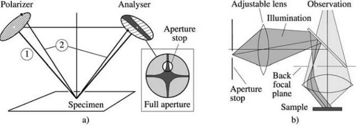
3.2.3. Kerr Microscopy... 56
3.2.3.1. The illumination Path ... 57
3.2.3.2 Domain observation ... 59
3.2.4. Study of magnetization reversal processes ... 60
3.3. Dynamics measurements ... 61
3.3.1. Ferromagnetic Resonance (FMR) ... 61
3.3.1.1. Experimental arrangement of FMR ... 63
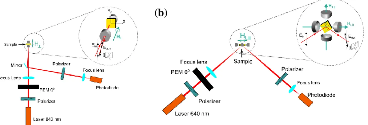
3.3.2. Brillouin Light scattering (BLS) spectroscopy ... 65
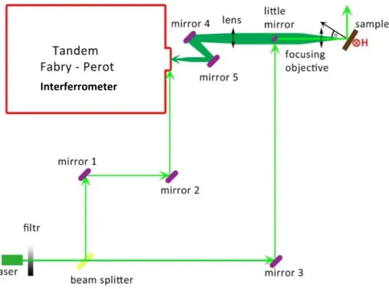
3.3.2.1. Experimental arrangement... 68
3.3.2.2. Tandem Fabry-Pérot (TFP) interferometer... 69
4. Results and Discussions ... 73
4.1. Fe60Al40 ... 74
4.1. Fe60Al40 ... 75
4.1.1. Sample fabrication ... 75
4.1.1.1. Uniformly irradiated thin films ... 75
4.1.1.2. Fabrication of 1D stripes ... 77
4.1.2. Statics measurements ... 80
6
4.1.3.1. Magnetization state ... 80
4.1.3.2. Magnetization reversal study ... 82
4.1.3.2. Magnetization reversal in reprogrammable 1D stripe ... 86
4.1.3.2.1. Magnetization reversal for uniformly irradiated stripe ... 86
4.1.3.2.2. Magnetization reversal study in 1D reprogrammable stripe ... 87
4.1.3. Study of magnetization dynamics ... 88
Summary ... 99
4.2. Patterned (antidot lattices) Py ... 101
4.2. Nanopatterns of Py ... 102 4.2.1. Sample fabrication ... 102 4.2.2. Structural analysis ... 103 4.2.2.1. SEM analysis ... 104 4.2.2.2. AFM analysis ... 105 4.2.3. Statics measurements ... 106 4.2.4. Dynamics measurements ... 117 4.2.4.1. FMR study ... 117 Summary ... 129
4.3. Thin films of Pt/Co/Pt ... 131
4.3.1. Sample fabrication:... 132 4.3.2. Statics measurements ... 133 4.3.2.1. PMOKE measurements ... 133 4.3.2.2. LMOKE measurements ... 137 4.3.3. Dynamics measurements ... 138 Summary ... 144 5. Conclusions ... 145 6. References ... 147 6. List of publications ... 157 Acknowledgements ... 160
7
Glossary
BLS Brillouin Light Scattering FMR Ferromagnetic Resonance FWHM Full width at half maximum hf High frequency
LL Landau-Lifshitz LLG Landau-Lifshitz-Gilbert MOKE Magneto-Optical Kerr Effect
LMOKE Longitudinal Magneto-Optical Kerr Effect PMOKE Perpendicular Magneto-Optical Kerr Effect MSSW Magnetostatic Surface Wave
MR Magnetization reversal Py Permalloy (Ni81Fe19)
VNA Vector network analyzer 1D One dimensional 2D Two dimensional MCs Magnonic crystals Antidot lattice ADL
EBL Electron beam lithography
CMOS complementary metal-oxide-semiconductor Spin waves SW
Py Permalloy
DUV Deep ultraviolet
DMI Dzyaloshinsky-Moriya interaction
DE Damon Eshbach
SSW Standing spin waves
PMA Perpendicular magnetic anisotropy GMR Giant magnetoresistance CVD Chemical vapor deposition PVD Physical vapor deposition PLD Pulse laser deposition MBE Molecular beam epitaxy LEED Low energy electron diffraction
RHEED Reflection high energy electron diffraction UHV Ultra-high vacuum
FIB Focus ion beam
VNA-FMR Vector network analyzer-ferromagnetic resonance
Hc Coercive field
H1eff Effective field
mr Magnetization remanence
B Vector of magnetic induction
d thickness
deff Effective thickness
f Precessional frequency
J Exchange integral
M = M/MS Reduced magnetization vector
MS Saturation magnetization
ω = 2πf Angular frequency
Hsat Saturation field
Ku Uniaxial anisotropy
Meff Effective magnetization
HR Reversal field
t1/2 Relaxation time
laser Wavelength of laser
g g-factor γ gyromagnetic ratio µB Bohr magneton µ0 Permeability A Exchange constant α Damping constant K Anisotropy constant lex Exchange length fDE Frequency of DE mode
fSSW Frequency of standing spin
waves
q Wave-number across the film
thickness
pd Pinning at certain depth
Symbols
8
1. Introduction
9
1.1. Introduction
The modern research on fundamental properties of materials is increasingly driven by their anticipated potential for technological applications. Due to their intricate nanostructures, extremely small length scale, low dimensionality, and interplay among constituents, they often present new and enhanced properties over their parent bulk materials. Recent progress on magnetism and magnetic materials has made nanostructures a particularly interesting class of materials for both scientific and technological applications such as sensors, patterned media, and novel magnetic properties [Mar03, She02, Bad06, Ake04, Stu03, Sko03]. Magnetic nanostructures can be fabricated by means of many advances fabrication techniques, e.g. electron beam lithography (EBL), deep ultraviolet lithography, focused ion beam patterning or ion beam etching, etc..
By modulating magnetic thin film properties in proper order, one can form one dimensional (1D), two dimensional (2D) magnonic crystals (MCs)-a new class of metamaterials with periodically modulated magnetic properties which due to unique properties of spin waves can offer new functionalities that are currently unavailable in e.g. photonic and electronic devices [Gie05, Gie07, Her04, Khi07, Khi08, Lee08, Pod05, Pod06, and Vas07] as magnonic devices are easily manipulated by the applied magnetic field. Moreover, magnetic nano-structures are non-volatile memory elements, and therefore, their integration will enable programmable devices with the ultrafast re-programming at the sub-nanosecond time scale. At remanence, a mono-domain nanomagnet with uniaxial magnetic anisotropy has two energy minima for opposing orientations of the magnetization M collinear with the easy axis. MCs can be also be designed via different quasi-static magnetic states of subcomponents of an MC or magnonic device. In general, to demonstrate the rich technological potential of magnonics, one has to design and to build nanoscale functional magnonic devices, in particular those suitable for monolithic integration into existing complementary metal-oxide-semiconductor (CMOS) circuits. In magnetic data storage media magnetic nano-structures have already been combined with nano- electronics (e.g. in read heads and magnetic random access memories) and optics (e.g. in magneto-optical disks). Hence, magnonic devices offer the integration with microwave electronics and photonic devices at the same time. Since for all practically relevant situations (at the GHz to THz frequency range), the wavelength of spin waves is several orders of magnitude shorter than
10
that of electromagnetic waves, magnonic devices offer better prospects for miniaturization at these frequencies.
Ferromagnetic metals show a spin wave (SW) damping that leads to decay lengths of typically several10µm. SW propagation in un-patterned Py was resolved over 80 µm [Kru10]. Along with Py nanostructures (dots), antidots structures (the reverse of isolated nanostructures) form another class of magnetic nanostructures in which arrays of holes are embedded into contiguous magnetic materials. Antidots are artificially engineered “defects” in an otherwise continuous film. The antidote lattice (ADL) has also been proposed as a competitor for high density storage media, with characteristics of high stability while avoiding the superparamagnetic limit [Cow97]. In the antidot lattices, spin waves propagate through the continuous ferromagnetic medium between the antidots and have much higher propagation velocity and longer propagation distance as compared to other for type of MCs such as lattice formed by dots or stripes. Due to the advances in the fabrication technology the proper arrangement of these antidots can lead to change in magnetic properties of the thin films in controllable manner [Ade08]. Such structures can be regarded as an example of two-dimensional (2D) artificial MCs [Khi08, Sch08]. Effect of antidot shape (square, circular, elliptical), size, interspacing distance, and arrangement (square lattice, honeycomb lattice, rhombic lattice) on statics (magnetization reversal), and dynamics of magnetization (spin waves) have been carried out by different techniques [Tri10, Tac10, Wan06, Gue02, Gue03, Yu03, Man15, Len11, and Dem13]. There is still quest to know: how ADL structures tune the magnetization reversal, and spin wave excitation in geometrically perturbed magnetic thin films.
It has been quite known that magnetic properties of the magnetic thin films can be further tailored by processing capabilities such as ion irradiations, which have proven itself a powerful tool to modify and tune magnetic properties [Fas04, Fas08 and Maz12]. In general ion induced changes are related to the deformation of the chemical structures, hence the magnetic phase which lowers the magnetic patterning which is highly important for bit patterned media. Conversely ions irradiation can be used to induce ferromagnetism in certain alloys through creating chemical disorder in such system [Fas08a, Bal14, Tah14, Tah15, Tah15a, Men09 and Sor06].
11
1.2. Objectives and structure of the thesis
Within the framework of this thesis, detailed study to understand the effects of geometry of the nano-patterns, and ion irradiation on the statics and dynamics of magnetization in Py antidots structures, and irradiated Fe60Al40 and Pt/Co/Pt thin films respectively is carried out.
The goals of the thesis were focused to the studies of:
1. Influence of complex antidot lattice geometry (from square lattice to wave-like patterns) on magnetic anisotropy, magnetization reversal mechanisms, and spin wave excitation spectra.
2. Effect of irradiation energy driven modification in Fe60Al40 thin films on combined
magnetic properties: static (evolution of magnetic domain structures, magnetization reversal mechanisms) and dynamic (spin waves excitations). A very recently it was demonstrated that discrete magnetic patterning can be achieved in such system [Bal14], which makes this it a potential candidate for MCs.
3. Role of 30 keV Ga+-ions fluence on spin wave excitations in irradiated Pt/Co/Pt ultrathin films. Recently [Maz12] has reported possibilities of induced magnetic anisotropy modifications through ion irradiation fluence.
This thesis is divided into seven chapters (introduction being the first chapter). In this chapter brief introduction related to the importance of magnetic nanostructures, their potential use in scientific research and depth of the pertinent issues has been presented.
Chapter 2 provides brief information about the magnetic moment, magnetic interactions,
magnetic anisotropy, magnetic domains, magnetization process, magnetization dynamics, and spin waves.
Chapter 3 comprises the overview of the experimental techniques such as sample fabrication,
and their characterization.
Chapter 4 comprises the results and discussion. This chapter is further divided into
sub-chapters depending on our study for different considered systems.
Chapter 4.1 We will show how energy of the irradiated ions is responsible for different
magnetization reversal processes and evolving of domains structure. We shall demonstrate how energy of the irradiated ions affects the spin wave excitations. The reprogramability of 1D stripe patterned by Ne+ ions will also be shown.
12
Chapter 4.2: Complexity effects of antidot lattice structures (from square lattice to wave-like
patterns) on magnetization reversal, magnetic anisotropy, and spin wave excitations will be presented. In order to provide better understanding the experimental results will be supported with MuMax calculations.
Chapter 4.3: In this section role of Ga+ irradiated ions fluence (F) on spin waves excitations in Pt/Co/Pt thin films will be presented.
Chapter 5 summarizes the work presented in this thesis.
All the concerned literature will be summarized in chapter 6.
Chapter 7 will be based on list of published work and work presented in the conferences.
13
2. Theory
14
2. Theory
2.1. Introduction to Magnetism
Magnetism is enhanced by the fact that the field still undergoes dynamic developments. Ever new magnetic phenomena continue to be discovered in conjunction with our ability to atomically engineer new materials. As in throughout history, today’s magnetism research remains closely tied to applications. It is therefore no surprise that some of the forefront research areas in magnetism today are driven by the “smaller and faster” mantra of advanced technology. The goal to develop, understand, and control the spin in metamaterials is furthermore accompanied by the development of new experimental techniques, that offer capabilities not afforded by conventional techniques.
2.1.1. Origin of Magnetic Moment
The magnetization of a matter is derived by electrons moving around the nucleus of an atom. The magnetism is related to spin angular momentum, orbital angular momentum and spin-orbit interactions angular momentum.
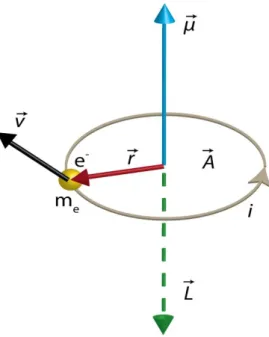
In classical electromagnetism the magnetic moment µ can be explained using the picture of a current loop. Assuming an electron is rotating from left to right on the table plane as shown in (Fig. 2.1). The rotating electron creates a current i on the circle with radius of r. The magnetic moment of a single electron is defined as:
𝜇⃗ = 𝑖. 𝐴⃗ (2.1)
Where, 𝐴⃗ is the circle area. The magnetic moment is written as follows by using the current
(-e = i . t), on(-e cycl(-e (2𝜋 = 𝑣. 𝑡) and angular momentum (𝐿 = 𝑚𝑒. 𝑣. 𝑟) definition.
Figure 2.1: Schematic representation of the precession of a single electron on the table plane.
15
𝜇⃗ = −2𝑚𝑒
𝑒𝐿⃗⃗ (2.2)
where 𝛾 = 𝑒 2𝑚
𝑒
⁄ and 𝐿⃗⃗ is the gyromagnetic (magneto-mechanical or magneto-gyric) ratio and the angular magnetic moment respectively. Therefore, the moment 𝜇⃗ can be described as:
𝜇⃗ = −𝛾𝐿⃗⃗ (2.3)
The time derivative of Eq. (2.3) gives us following equation (𝛾 is constant):
1 𝛾 𝑑𝜇⃗⃗⃗ 𝑑𝑡 = 𝑑𝐿⃗⃗ 𝑑𝑡 = 𝜏⃗ (2.4)
This equation is related to 𝜏⃗ = 𝑑𝐿⃗⃗ 𝑑𝑡⁄ in two dimensional motion on the plane and 𝐹⃗ = 𝑑𝑃⃗⃗ 𝑑𝑡⁄ in one dimensional motion. The equation of motion of magnetic moment in an external field will be express as:
1 𝛾
𝑑𝜇⃗⃗⃗
𝑑𝑡 = 𝜇⃗ × 𝐻⃗⃗⃗ (2.5)
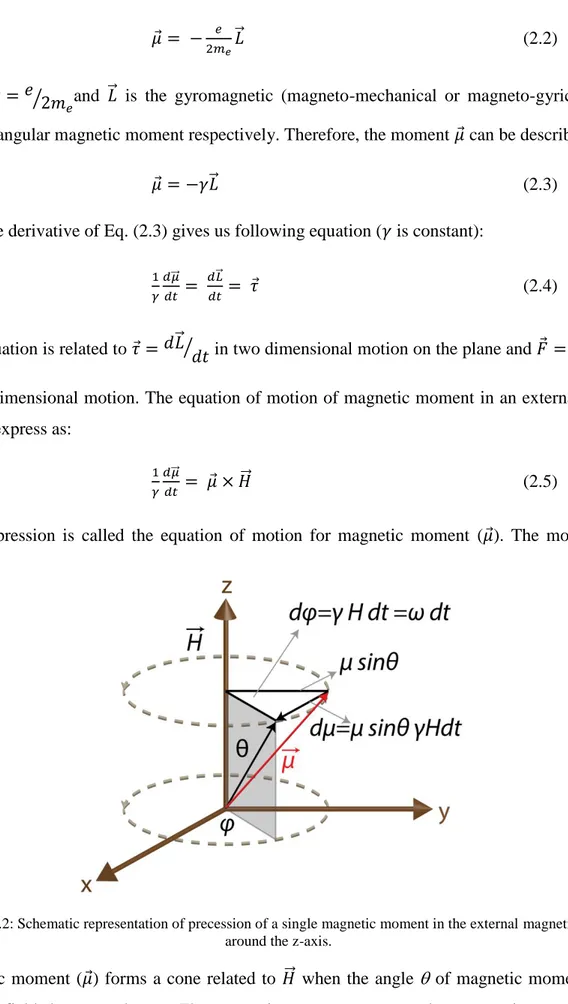
This expression is called the equation of motion for magnetic moment (𝜇⃗). The motion of
magnetic moment (𝜇⃗) forms a cone related to 𝐻⃗⃗⃗ when the angle of magnetic moment and external field does not change. The magnetic moment vector makes precession movement
Figure 2.2: Schematic representation of precession of a single magnetic moment in the external magnetic field around the z-axis.
16
around external field at a frequency of 𝛾𝐻⁄ . This frequency, 𝑣 = 𝜔 2𝜋2𝜋 ⁄ = 𝛾𝐻 2𝜋⁄ , is called the Larmor frequency. In general this frequency used the form (𝜔 = 𝛾𝐻) in the literature.
The energy of a magnetic moment is given by:
𝐸 = −𝜇𝑜𝜇. 𝑯 = −𝜇𝑜𝜇𝐻𝑐𝑜𝑠𝜃 (2.6)
with being the angle between the magnetic moment and an external magnetic field H and
o the magnetic permeability of free space.
The magnitude of the magnetization M is defined as the total magnetic moment per volume unit:
𝑀 = 𝜇𝑁𝑉 (2.7)
Usually, it is given on a length scale which is large enough that an averaging over at least several atomic magnetic moments is carried out. Under this condition the magnetization can be considered as a smoothly varying vector field. In vacuum no magnetization M occurs.
The microscopic origin of magnetism can be described by quantum mechanical treatment. In solid states, magnetism mainly originates from the magnetic properties of the electrons. Partly, the magnetic moment of the electron is mediated by the angular momentum associated with its motion around the nucleus. The component of this orbital angular momentum along a distinct axis (usually one chooses the z-axis) is defined by the quantum number ml and is given by mlħ where ħ is Planck’s constant divided by 2. Associated with
this angular moment the electron has a magnetic moment along the z-axis of
−𝑔𝑙𝑚𝑙𝜇𝐵, (2.8)
where 𝜇𝐵 = 𝑒ℏ (2𝑚 𝑒)
⁄ is the Bohr magneton and 𝑔𝑙being the 𝑔-factor for the orbital momentum. Moreover, in addition to the orbital angular momentum the electron possesses an intrinsic momentum called spin. It is accounted for by the spin quantum number m s = ±1/2, which defines the component of the spin angular momentum along a fixed direction (again the z-axis) given by 𝑚𝑠ℏ. The associated magnetic moment along the z-axis reads
17
𝑔𝑠𝑚𝑠𝜇𝐵, (2.9)
where 𝑔𝑠 = 2 is the 𝑔-factor of the electron spin.
Since magnetism is a collective phenomenon, the magnetic moments need to communicate with each other. The mechanisms responsible for the different possible interactions are described in the following subsections.
2.2. Magnetic interactions
There are several sources of magnetic interactions by emphasizing ferromagnetic ordering since the ferromagnetism is the subject of this research project.
2.2.1. Magnetic dipolar interaction
Consider two magnetic dipoles µ1 and µ2, each immersed in the magnetic field generated
by the other dipole. In this case the corresponding magnetic energy reads [Mat08].
𝐸𝑑𝑖𝑝𝑜𝑙𝑒 = 4𝜋𝑟𝜇𝑜3[𝜇1. 𝜇2−𝑟32(𝜇1. 𝑟)(𝜇2. 𝑟)], (2.10)
where o is the permeability. Since r is the vector connecting the two dipoles, the energy
decreases with the 3rd order of their distance. For an estimation of this energy we choose typical values with µ1 = µ2 = 1 µB and r = 2Å. Additionally, we assume µ1µ2 and µr.
This situation results in an energy of:
𝐸 = 𝜇𝑜𝜇𝐵2
2𝜋𝑟3 = 2.1 × 10⁻²⁴𝐽 (2.11)
The corresponding temperature (E = kT) is far below 1K. But, the order temperature typically reaches values of several 100K for a lot of ferromagnetic materials. Therefore, the magnetic dipole interaction is too small to cause ferromagnetism. However, this interaction is accountable for effects such as demagnetizing field and spin waves in the long wave length regime.
2.2.2. Exchange interaction
Magnetism can be divided into two groups, A and group B. In group A there is no interaction between individual moments and each moment acts independently of the others.
Group B consists of the magnetic materials most people are familiar with, like iron, nickel. Magnetism occurs on these materials because the magnetic moments couple to one
18
another and form magnetically ordered states. The coupling, which is quantum mechanical in nature is known as exchange interaction and is rooted in the overlap of electrons in conjuction with Pauli’s exclusion principle. Exchange interactions lie at the heart of the phenomenon of long range magnetic order. Exchange interactions are nothing more than electrostatic interactions, arising because charges of the same sign cost energy when they are close together and save energy when they are apart. Whether it is a ferromagnet, Antiferromagnet of ferrimaget the exchange interaction between the neighboring magnetic ions will force the individual moments into parallel (ferromagnetic) or antiparallel (antiferromagnetic) alignment with their neighbors. There are following types of exchange which are currently believed to exit are:
2.2.2.1. Direct Exchange
If the electrons on neighboring magnetic atoms interact via an exchange interaction, this is known as direct exchange. This is because the exchange interaction proceeds directly without the need for an intermediary. Though this seems the most obvious route for the exchange interaction to take, the reality in physical situations is rarely that simple.
Very often direct exchange cannot be an important mechanism in controlling the magnetic properties because there is insufficient direct overlap between neighboring magnetic orbitals. For example, in rare earths the 4f electrons are strongly localized and lie very close to the nucleus, with little probability density extending significantly further than about a tenth of the interatomic spacing. This means that the direct exchange interaction is unlikely to be very effective in rare earths. Even in transition metals, such as Fe, Co and Ni, where the 3d orbitals extend further from the nucleus, it is extremely difficult to justify why direct exchange should lead to the observed magnetic properties. These materials are metals which means that the role of the conduction electrons should not be neglected, and a correct description needs to
(a) (b)
Figure 2.3: (a) Antiprallel alignment for small interatomic distances, (b) Parallel alignment for large interatomic distances.
19
take account of both the localized and band character of the electrons. Thus in many magnetic materials it is necessary to consider some kind of indirect exchange interaction.
The exchange energy forms an important part of the total energy of many molecules and of the covalent bond in many solids. Heisenberg showed that it also plays a decisive role in ferromagnetism. This indeed is an alternative way of formulating Pauli’s exclusion principle, since it implies the probability to find two electrons with parallel spins in the same state to vanish. Therefore, the Coulomb energy of electrons with parallel spins is lowered on account of their spatial separation. The corresponding exchange energy of two electrons with spin operators 𝑆̂ and 𝑆1 ̂ can be expressed as 2
𝐸𝑒𝑥= −2𝐽12𝑆1. 𝑆2 = −2𝐽𝑆1𝑆2𝑐𝑜𝑠𝜑 (2.12)
where J12 is a particular integral, called the exchange integral, and 𝜑 is the angle between the
spins. For J12 > 0 the interaction causes parallel alignment of the spins, which corresponds to
ferromagnetic order. In a continuum approximation of the crystal lattice, the exchange energy of a cubic crystal is given by:
𝐸𝑒𝑥= 𝐴 ∫ 𝑑𝑉(∇𝑚)2 (2.13)
With the exchange constant A = 2 JS2 p/a and the normalized magnetization m = M/MS and
MS being the magnetization vector and the saturation magnetization respectively. The
exchange integral is J, the distance between the nearest neighbors is a, and the number of sites in the unit cell is denoted by p. Since the exchange constant depends on the overlap of the
20
single electron wave functions, which is taken into account by a, J generally vanishes except for neighboring electrons.
The Bethe-Slater curve represents the magnitude of direct exchange as a function of interatomic distances. The curve of Fig. 2.4 [Cul09] can be applied to a series of different elements if we compute ra/r3d from their known atom diameters and shell radii. The points so
found lie on the curve as shown, and the curve correctly separates Fe, Co, and Ni from Mn and the next lighter elements in the first transition series. (Mn is antiferromagnetic below 95K, and Cr, the next lighter element, is antiferromagnetic below 37oC; above these temperatures they are both paramagnetic.) Although the theory behind the Bethe–Slater curve has received much criticism, the curve does suggest an explanation of some otherwise puzzling facts. Thus ferromagnetic alloys can be made of elements which are not in themselves ferromagnetic; examples of these are MnBi and the Heusler alloys, which have approximate compositions Cu2 MnSn and Cu2MnAl. Because the manganese atoms are
farther apart in these alloys than in pure manganese, ra/r3d becomes large enough to make the
exchange interaction positive.
Consequently, the exchange interaction is only very short ranged. However, due its magnitude which is of the order of 10−2 eV, it can exclusively account for magnetic long range ordering and causes a mutual alignment of the permanent magnetic moments below a critical temperature.
2.2.2.2. Indirect exchange in Metals
Indirect exchange couples moments over relatively large distances. It is the dominated exchange interaction in metals, where there is little or no direct overlap between neighboring electrons. It therefore acts through an intermediary, which in metals are conduction electrons (itinerant electrons). This type of exchange is better known as RKKY (the initial letters of the surnames of the discoverers of the effect, Ruderman, Kittel, Kasuya and Yosida) interaction. A magnetic ion induces a spin polarization in the conduction electrons in its neighborhood. This spin polarization in the itinerant electron is felt by the moments of other magnetic ions within the range leading to an indirect exchange coupling.
The coupling takes the form of an r-dependent exchange interaction JRKKY (r) given by
𝐽𝑅𝐾𝐾𝑌(𝑟) ∝ 𝑐𝑜𝑠(2𝑘𝐹𝑟)
21
at large r (assuming a spherical Fermi surface of radius kF). The interaction is long range and
has an oscillatory dependence on the distance between the magnetic moments shown in Fig.
(2.5). Hence depending on the separation it may be either ferromagnetic or antiferromagnetic. The coupling is oscillatory with wavelength /kF because of the sharpness of the Fermi
surface.
2.2.2.3. Indirect exchange in ionic solids: superexchange
A number of ionic solids, including some oxides and fluorides, have magnetic ground states. For example, MnO and MnF2 are both antiferromagnets, though this observation
appears at first sight rather surprising because there is no direct overlap between the electrons
on Mn2+ ions in each system. The exchange interaction is normally very short-ranged so that the longer- ranged interaction that is operating in this case must be in some sense 'super'.
JRKKY
Interatomic distance a
Figure 2.5: The coefficient of indirect (RKKY) exchange versus the interatomic spacing a.
Fig. 2.6: Occurrence of a super exchange interaction in a magnetic oxide. The arrows represent the spins of the electrons being involved into the interaction between the metal (M) and oxygen (O) atom. Image
22
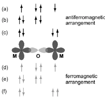
For example in the case of antiferromagnetic ionic solid MnO, each Mn2+ ion exhibits 5 electrons in its d shell with all spins being parallel due to Hund’s rule. The O2− ions possess electrons in p orbitals which are fully occupied with their spins aligned antiparallel. There are two possibilities for the relative alignment of the spins in neighboring Mn atoms. A parallel alignment leads to a ferromagnetic arrangement whereas an antiparallel alignment causes an antiferromagnetic arrangement. That configuration is energetically favored which allows a delocalization of the involved electrons due to a lowering of the kinetic energy (see Fig. 2.6) [Blu01]. In the antiferromagnetic case the electrons with their ground state given in (a) can be exchanged via excited states shown in (b) and (c) leading to a delocalization. For ferromagnetic alignment with the corresponding ground state presented in (d) the Pauli Exclusion Principle forbids the arrangements shown in (e) and (f). Thus, no delocalization occurs. Therefore, the antiferromagnetic coupling between two Mn atoms is energetically favored. It is important that the electrons of the oxygen atom are located within the same orbital, i.e. the atom must connect the two Mn atoms.
2.2.2.4. Double exchange
In some oxides, it is possible to have a ferromagnetic exchange interaction which
Fig. 2.7: Double exchange mechanism gives ferromagnetic coupling between Mn3+ and Mn4+ ions participating in electron transfer. The single-centre exchange interaction favors hopping if (a) neighboring ions are ferromagnetically aligned and not if (b) neighboring ions are antiferromagnetically aligned. Image is adopted
23
occurs because the magnetic ion can show mixed valency, that is it can exist in more than one oxidation state. Examples of this include compounds containing the Mn ion which can exist in oxidation state 3 or 4, i.e. as Mn3+ or Mn4+.
The ferromagnetic alignment is due to the double exchange mechanism which can be understood with reference to Fig. 2.7 [Blu01]. The eg electron on a Mn3+ ion can hop to a
neighboring site only if there is a vacancy there of the same spin (since hopping proceeds without spin-flip of the hopping electron). If the neighbor is a Mn4+ which has no electrons in its eg shell, this should present no problem. However, there is a strong single-centre (Hund's
rule number 1) exchange interaction between the eg electron and the three electrons in the t2g
level which wants to keep them all aligned. Thus it is not energetically favorable for an eg
electron to hop to a neighboring ion in which the t2g spins will be antiparallel to the eg electron
(Fig. 2.7(b)). Ferromagnetic alignment of neighboring ions is therefore required to maintain the high-spin arrangement on both the donating and receiving ion. Because the ability to hop gives a kinetic energy saving, allowing the hopping process shown in Fig. 2.7(a) reduces the overall energy. Thus the system ferromagnetically aligns to save energy. Moreover, the ferromagnetic alignment then allows the eg electrons to hop through the crystal and the
material becomes metallic.
2.2.2.5. Anisotropic exchange interaction
It is also possible for the spin-orbit interaction to play a role in a similar manner to that of the oxygen atom in superexchange. Here the excited state is not connected with oxygen but is produced by the spin-orbit interaction in one of the magnetic ions. There is then an exchange interaction between the excited state of one ion and the ground state of the other ion. This is known as the anisotropic exchange interaction, or also as the Dzyaloshinsky-Moriya
interaction (DMI). When acting between two spins S1 and S2 it leads to a term in the
Hamiltonian, ĤDM equal to: [Blu01]
ĤDM = D. S1S2 (2.15)
The vector D vanishes when the crystal field has an inversion symmetry with respect to the centre between the two magnetic ions. However, in general D may not vanish and then will lie parallel or perpendicular to the line connecting the two spins, depending on the symmetry. The form of the interaction is such that it tries to force S1 and S2 to be at right angles in a
24
negative. Its effect is therefore very often to cant (i.e. slightly rotate) the spins by a small angle. It commonly occurs in antiferromagnets and then results in a small ferromagnetic component of the moments which is produced perpendicular to the spin-axis of the antiferromagnet. The effect is known as weak ferromagnetism. It is found in, for example, a-Fe2O3, MnCO3 and CoCO3.
2.3. The Energy Functional of a Magnet
The total internal magnetic field Heff acting on the magnetic moments inside a solid results
from the functional derivative of the total energy density Etot = Etot /V with respect to the
reduced magnetization m(r) = M (r)/MS.
𝐻𝑒𝑓𝑓 = −𝜇1
𝑜 𝛿𝐸𝑡𝑜𝑡
𝛿𝒎 , (2.16)
where V is the sample volume. The free energy density of a magnetic system is given by
𝐸𝑡𝑜𝑡 = 𝐸𝑧𝑒𝑒+ 𝐸𝑎𝑛𝑖+ 𝐸𝑑𝑒𝑚+ 𝐸𝑒𝑥 (2.17)
where Ezee represents the Zeeman energy, Eani the anisotropy, Edem the demagnetizing, and Eex
the exchange energy density.
2.3.1. Zeeman Energy
The Zeeman term arises from the interaction of the magnetization M with an external field Ho and represented by the following equation
𝐸𝑧𝑒𝑒 =𝑉1∫ 𝑑𝑉 𝑀 . 𝐻𝑜 (2.18)
It favors parallel alignment of the magnetization along the external field direction.
2.3.1.1. Magnetocrystalline anisotropy
The most important type of anisotropy is the magneto crystalline anisotropy which is caused by the spin orbit interaction of the electrons. The electron orbitals are linked to the crystallographic structure. Due to their interaction with the spins they make the latter prefer to align along well defined crystallographic axes. Therefore, there are directions in space which a magnetic material is easier to magnetize in than in other ones (easy axes or easy magnetization axes). The spin-orbit interaction can be evaluated from basic principles. However, it is easier to use phenomenological expressions (power series expansions that take into account the crystal symmetry) and take the coefficients from experiment.
25
In cubic systems the energy density due to crystal anisotropy reads
𝐸𝑎𝑛𝑖 = 𝐾𝑜+ 𝐾1(𝛼𝑥2𝛼
𝑦2+ 𝛼𝑦2𝛼𝑧2+ 𝛼𝑧2𝛼𝑥2) + 𝐾2𝛼𝑥2𝛼𝑦2𝛼𝑧2, (2.19)
where i are the directional cosines of the normalized magnetization m with respect to the
Cartesian axes of the lattice. Ki are the magnetocrystalline anisotropy constants, Ko, K1, and
K2 are the crystalline anisotropy constants of zero, first and second order, respectively. In
addition to the intrinsic ordering arising from the crystal lattice, atomic ordering may also be caused by surfaces and interface and hence is of particular importance in confined magnetic system. For crystals exhibiting uniaxial anisotropy, the energy density is
𝐸𝑎𝑛𝑖 = 𝐾𝑈𝛼𝑥2, (2.20)
with the uniaxial anisotropy constant KU.
2.3.2. Anisotropy Energy
Magnetic anisotropy is the directional dependence of material’s magnetic properties. In the absence of external magnetic field, a magnetically isotropic material has no preferential directions for its magnetic moment while a magnetically anisotropic material will align its magnetic moments with one of the easy axis (the energetically favorable axis in which spontaneous magnetization aligns determined by the source of magnetic anisotropy). There could be several sources of magnetic anisotropy. Beside the stress anisotropy (also called magnetostriction), and induced magnetic anisotropy other sources such as magnetocrystalline anisotropy, shape anisotropy (demagnetizing or stray field), and surface and interface anisotropy are discussed in the following section being related to area of present study.
2.3.2.1. Demagnetizing Energy
Polycrystalline samples without a preferred orientation of the grains do not possess any magneto crystalline anisotropy. But, an overall isotropic behavior concerning the energy being needed to magnetize it along an arbitrary direction is only given for a spherical shape. If the sample is not spherical then one or more specific directions occur which represent easy magnetization axes which are solely caused by the shape. This phenomenon is known as shape anisotropy. In order to get a deeper insight we have to deal with the stray and demagnetizing field of a sample.
26
The relationship 𝐵 = 𝜇𝑜(𝐻 + 𝑀) only holds inside an infinite system. A finite system exhibits poles at its surfaces which leads to a stray field outside the sample. This occurrence of a stray field results in demagnetizing field inside the sample.
The energy of a sample in its own stray field is given by the stray field energy Edem
𝐸𝑑𝑒𝑚 = −12∫ 𝜇𝑜𝑀. 𝐻𝑑𝑒𝑚 𝑑𝑉 (2.21)
The expression for the demagnetizing field of an arbitrary shaped element generally constitutes a very complex function of position. It is however, uniform in the case of an homogenously magnetized ellipsoid (possesses a constant demagnetizing field Hdem) which is
given by:
Hdem = -NM (2.22)
with N being the demagnetizing tensor. Thus, the stray field energy (demagnetizing energy) amounts to:
𝐸𝑑𝑒𝑚 = 1 2⁄ . 𝜇𝑜∫ 𝑀𝑁𝑀𝑑𝑉 (2.23)
𝐸𝑑𝑒𝑚 = 1 2⁄ 𝑉𝜇𝑜𝑀𝑁𝑀 (2.24)
with V being the volume of the sample. N is a diagonal tensor if the semi axis a, b, and c of the ellipsoid represents the axes of the coordination system. Then, the trace is given by
trN = 1 (2.25)
An arbitrary direction of the magnetization with respect to the semi axes can be characterized by the direction cosine a. b, and c. The tensor is given by:
𝑁 = (
𝑁𝑎 0 0
0 𝑁𝑏 0 0 0 𝑁𝑐
) (2.26)
and the demagnetizing energy per volume amounts to”
𝐸𝑑𝑒𝑚 = 1 2⁄ . 𝜇0. 𝑀2(𝑁𝑎𝛼𝑎2+ 𝑁𝑏𝛼𝑏2+ 𝑁𝑐𝛼𝑐2) (2.27)
27 𝑁 = ( 1 3 ⁄ 0 0 0 1⁄3 0 0 0 1⁄ )3 (2.28)
and the demagnetizing field energy density to:
𝐸𝑑𝑒𝑚 = 1 2⁄ . 𝜇𝑜𝑀2. 1 3⁄ (𝛼 𝑎 2 + 𝛼
𝑏2+ 𝛼𝑐2) (2.29)
𝐸𝑑𝑒𝑚 = 1 6⁄ . 𝜇𝑜𝑀2 (2.30)
For an infinitely extended and very thin plate, we have a = b = , and
𝑁 = ( 1 2 ⁄ 0 0 0 1⁄2 0 0 0 1⁄ )2 (2.31)
Now, the demagnetizing field energy density amounts to:
𝐸𝑑𝑒𝑚 = 1 2⁄ . 𝜇𝑜𝑀2𝑐𝑜𝑠2𝜃 (2.32)
This results is important for thin magnetic films and multilayers. Equation (2.32) can be rewritten as:
𝐸𝑑𝑒𝑚 = 𝐾𝑜+ 𝐾𝑠ℎ𝑎𝑝𝑒𝑉 𝑠𝑖𝑛2𝜃 (2.33)
with 𝐾𝑠ℎ𝑎𝑝𝑒 𝑉 ∝ −𝑀2 < 0. The demagnetizing field energy reaches its minimum value at =
90o. This means that shape anisotropy favors a magnetization direction parallel to the surface, i.e. within the film plane.
2.3.2.2. Surface and interface anisotropy
Due to the broken symmetry at interfaces the anisotropy energy contains terms with lower order in α which are forbidden for three-dimensional systems. Therefore, each effective anisotropy constant Keff is divided into two parts, first term on right hand side describing the volume and second term the surface contribution
28
with KV being the volume dependent magneto crystalline anisotropy constant and KS the surface dependent magneto crystalline anisotropy constant. The factor of two is due to the creation of two surfaces. The second term exhibits an inverse dependence on the thickness d of the system. Thus, it is only important for thin films.
In order to illustrate the influence of the surface anisotropy we will discuss the so-called “spin reorientation transition” (SRT). Rewriting (2.34) results in:
𝑑. 𝐾𝑒𝑓𝑓 = 𝑑. 𝐾𝑉 + 2𝐾𝑆 (2.35)
Plotting this dependence as a d . Keff diagram allows to determine KV as the slope of the resulting line and 2KS as the zero-crossing which is exemplarily shown for a thin Co layer with variable thickness d on a Pd substrate (Fig. 2.8). Due to the shape anisotropy KV is negative. This can directly be seen by the negative slope which results in an in-plane magnetization. The zero-crossing occurs at a positive value KS. This leads to a critical thickness dc:
𝑑𝑐 = −2𝐾𝐾𝑉𝑆 (2.36)
with d < dc : perpendicular magnetization and for d > dc : in-plane magnetization due to the
change of sign of Keff.
Thus, the volume contribution always dominates for thick films with a magnetization
Fig. 2.8: Magnetic anisotropy of a Co thin film layer in a Co/Pd multilayer as a function of the Co thickness
29
being within the film plane. The relative amount of the surface contribution increases with decreasing thickness followed by a spin reorientation transition towards the surface normal below dc.
2.3.3. Exchange Energy
The exchange term has already been discussed above in section 2.2.2, equation (2.13). The corresponding energy density reads:
𝜀𝑒𝑥= 𝐴 ∫ 𝑑𝑉(∇𝑚)2 (2.37)
2.4. Magnetic Domains
Since the beginning of the last century, it is a well known fact that the magnetization is not uniform in a ferromagnetic material, but possesses a number of small regions (“magnetic” domains) with different orientation of magnetization. This domain configuration minimizes the stray field energy. Within each domain, the magnetic moments are aligned parallel to each other and point into one direction of the preferential directions that are determined by the magnetic field anisotropies in the absence of an applied external magnetic field. Domains are separated by domain walls.
These considerations allow to describe a lot of properties of different magnetic systems. Two examples are:
1. In soft magnetic materials smallest external fields (≈10−6T) are sufficient to reach saturation magnetization (μ0M≈1 T) by application of a very week magnetic field (as
low as 10-6T). Such low applied fields would have negligible effect on a paramagnet. The large effect in the ferromagnetic specimen is because the external field does not need to order all magnetic moments macroscopically (because in each domain they are
(a)
(b)
30
already ordered) but has to align the domains. Thus, a movement of domain walls only occurs which requires low energy.
2. It is possible that ferromagnetic materials exhibit a vanishing total magnetization M= 0 below the critical temperature without applying an external field. In this situation each domain still possesses a saturated magnetization but due to the different orientations the total magnetization amounts to zero.
2.4.1. Domain walls
The change of the magnetization direction between the adjacent domains does not occur
abruptly but is characterized by a slight tilt of the microscopic magnetic moments in the boundary regions. These boundary regions are several tens of nanometers wide and called domain walls. The domain walls can be classified by the angle of the magnetization between neighbored domains with the wall as boundary. A large variety of domain patterns exists depending on the specific properties of the ferromagnetic sample under investigation [Hub09]. A 180o domain wall represents the boundary between two domains with opposite magnetization (see Fig. 2.9a) and 90o wall domain wall represents the boundary between two domains with magnetization being perpendicular to each other (see Fig. 2.9b). A 180o domain wall is a Bloch wall (Fig. 2.10a) in which the magnetization rotates in a plane parallel to the plane of the wall. Another possible configuration is the Néel wall (Fig. 2.10b) where rotation of the magnetization takes place in a plane which is perpendicular to the plane of the domain wall [Bat08]. Bloch walls are more common in bulk-like thick films, while Néel walls are often observed in thin films (Fig. 2.11), where a surface stray field is avoided by the rotation of the moments within the surface plane. The width of a domain wall is determined by the exchange and the anisotropy energy [Hub09].
31
2.5. Magnetization processes
Magnetization processes are sensitive to the structures of magnetic materials. The existence of domains is hinted at by the observation that some magnetic properties, and in particular, coercivity and remanence. However, it must be noted that the coercivity is not an intrinsic magnetic property, which means that the value of the coercivity depends not only on the chemical composition, the temperature, and the magnetic anisotropy, but also strongly on the microstructure of the material [Wec87, Sch87, Mis87, Sch88, Mis88, Sag87, Ram88 and Fid96]. The necessary interplay between the microstructure and the intrinsic magnetic properties for the existence of coercivity in a given material is in general an intricate process. The understanding of the mechanisms of coercivity is essential for further improving hard magnetic properties. There are various methods of increasing or decreasing the coercivity of magnetic materials, which involve controlling the magnetic domains within the material. Depending on the Hc different regions can be classified:
1. Multidomain (MD). Magnetization changes by domain wall motion.
2. Single domain (SD). At critical thickness the system behaves as single domain and at this point coercivity reaches a maximum value. But this critical thickness coercivity decreses again but this time due to the randomizing effects of thermal energy.
2.5.1. Magnetic parameters
In an ideal crystal which does not contain any defects the magnetization of a demagnetized ferromagnet starts with reversible domain wall movements. This process ends when all domain walls are annihilated or all walls are oriented perpendicularly to the external magnetic field. If this is the only process until saturation is reached we obtain a magnetization as a function of the external magnetic field which is shown in Fig. 2.12.
Figure 2.11: The Néel wall is energetically favorable in thin film systems exhibiting only a small thickness d with an in-plane magnetization due to the avoidance of stray fields
32
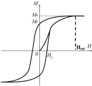
One can see that initially magnetization curve increases with the increase in the applied external field to demagnetized sample. In the first quadrant the magnetization and the applied field are both positive, i.e they are in the same direction. The magnetization increases initially by the growth of favorably oriented domains, which will be magnetized in the easy direction of the crystal. When the magnetization can increase no further by the growth of domains, the direction of magnetization of the domains then rotates away from the easy axis to align with the field. When all of the domains have fully aligned with the applied field saturation is reached and the magnetization cannot increase further. If the field is removed the magnetization returns to the y-axis (i.e., H = 0), and the domains will return to their easy direction of magnetization, resulting in a decrease in the overall magnetization. If the direction of applied field is reversed (i.e., to the negative direction) then the magnetization will follow the solid line into the second quadrant. The magnetization will only decrease after a sufficiently high field is applied to: (1) nucleate and grow domains favorably oriented with respect to the applied field or (2) rotate the direction of magnetization of the domains towards the applied field. After applying a high enough field the magnetization reaches its saturation value in the negative direction. If the applied field is then decreased and again applied in the positive direction then the full hysteresis loop is plotted. If the field is repeatedly switched from positive to negative directions and is of sufficient magnitude then the magnetization will cycle around the hysteresis loop in an anti-clockwise direction. The area contained within the
Hsat
Figure 2.12: A typical magnetic hysteresis loop for a ferromagnetic material. Saturation magnetization (MS), remanence (Mr), coercivity (Hc), and saturation field Hsat are illustrated on the curve.
33
loop indicates the amount of energy absorbed by the material during each cycle of the hysteresis loop.
The hysteresis loop is a means of characterizing magnetic materials, and various parameters can be determined from it. From the first quadrant (Fig. 2.12) the saturation magnetization, MS can be measured. Most of the useful information, however, can be derived
from the second quadrant of the loop, and, indeed, it is sometimes conventional only to show this quadrant. The magnetization retained by the magnet after the magnetizing field has been removed is called the remanence, Mr. The reverse field required to bring the magnetization to
zero is called the coercivity (Hc).
2.5.2. Magnetization reversal process
Magnetization reversal may be realized by changing applied field or by thermal activation. At constant field, thermal activation alone may lead to significant variation of magnetization in some cases. Time dependence of magnetization under constant field is referred as magnetic viscosity or magnetic aftereffect. The magnetic viscosity due to thermal activation is general properties of all ferromagnetic materials. Two magnetization reversal processes can be distinguished based on coercivity measurements. The first one is controlled by nucleation of reversed domains. The magnetization reversal is realized by spontaneous
expansion of these nucleated domain walls. Compared to nucleation, the propagation of the
Figure 1.14: Magnetization reversal curve for nucleation dominated (filled black squares) and domain wall motion dominated (filled red circles).
Figure 2.13: Time dependence magnetization relaxation curves: nucleation dominated (Black), and domain wall propagation (Red) reproduced from Fatuzzo and Lubrune model [Fat62, Lab89].
34
reversed domains occurs much easier. The other coercivity mechanism is controlled by the domain-wall propagation process. The domain wall is pinned by crystallographic defects or nonmagnetic precipitates (pinning centers). The magnetization reversal can only be realized by overcoming the maximum pinning force. The magnetization reversal processes can be described through the model (MR curves) proposed by Fatuzzo and Labrune [Fat62, Lab89] see (Fig. 2.13) in which two curves describe the two MR mechanisms. MR is processed through the curve (filled black squares) for nucleation dominated and the curve (filled red circles) domain wall motion dominated. More details are described in the appendix.
2.6. Magnetization Dynamics
When a magnetic material is exposed to an external magnetic field, its magnetic
moments tend to align themselves along the external field to minimize their energy. The kinetic motion of the magnetic moments disturbs this alignment. Therefore, the moments do not align themselves directly to the magnetic field; instead, they execute a precessional motion around the direction of the external field. The precession of magnetic moments is referred to as magnetization dynamics. The crucial difference of magnetization dynamics compared to static phenomena (usually in the millisecond time range) is the time scale on which the magnetic system is disturbed by an external stimulus and of course on which time scale one in turn observes its response. When applying quasi static fields to a magnetic system, the magnetization appears to be always in equilibrium since the dynamic processes happen on the nanosecond timescale or faster. In contrast, when applying alternating magnetic
Figure 2.14: The precessional motion of the magnetization around the effective magnetic field direction, governed by the Landau-Lifshitz-Gilbert equation (2.43).The torque −γM × Beff provides the rotational motion
around Beff while the Gilbert damping term forces the magnetization to be aligned along the effective field Beff.
35
fields with a frequency equal to the resonance frequency of the system, the magnetization configuration is resonantly disturbed from its equilibrium position. This behavior of magnetization under the influence of an external magnetic field is described phenomenologically by the Landau-Lifshitz and Gilbert equation of motion [Gil04].
The Landau-Lifshitz-Gilbert (LLG) equation is a torque equation which was first introduced by Lev Landau and Evgeny Lifshitz in 1935 as Landau-Lifshitz equation [Lan35]. The Landau-Lifshitz (LL) equation was a damping-free equation. Later, Gilbert modified it by inserting a magnetic damping term [Gil04]. In this section, first the LL equation will be derived by a semiclassical approach. Later, this equation will be modified by introducing the Gilbert damping term.
When a magnetic moment µm is placed in an effective magnetic field Beff, it
experiences a torque:
= µm × Beff (2.38)
In a semiclassical approach, the magnetic moment µm of an atom can be written in
terms of its angular momentum J as
𝜇𝑚 = −𝑔𝜇ℏ𝐵𝐽 = −𝛾𝐽 (2.39)
where = 𝑔𝜇𝐵⁄ is the gyromagnetic ratio. As ℏ = dJ/dt, Eq. (2.38) can be re-written as 𝑑𝐽 𝑑𝑡 = − 1 𝛾 𝑑𝜇𝑚 𝑑𝑡 = 𝜇𝑚× 𝐵𝑒𝑓𝑓 (2.40)
In the continuum limit, the atom magnetic moment can be replaced by the macroscopic magnetization M resulting in the equation of motion, i.e, Landau-Lifshitz (LL) equation:
𝑑𝑀
𝑑𝑡 = −𝜇𝑜𝛾𝑀 × 𝐵𝑒𝑓𝑓 (2.41)
Here, the effective magnetic field Beff is a sum of all external and internal magnetic fields:
36
Here, B0 is the static component of the applied magnetic field while BM(t) is the dynamic
component. Bex is a magnetic field originating from the exchange interaction. Bdem represents
the demagnetization field created by the dipolar interaction of magnetic surface and volume charges. The field Bani includes all kinds of anisotropic fields like shape anisotropy,
crystalline anisotropy, etc.
The physical meaning of Eq. (2.41) explores two important features of the equation of motion. A dot-product of Eq. (2.41) with M results that the magnitude of M is conserved. Secondly, a dot product with Beff concludes that the orientation of M with respect to Beff will
not vary over time. Further, the system is non-dissipative which means that the magnetization will continue to precess for infinitely long time. Definitely, in the real world no such system exists. To rectify this issue, Gilbert [Lan35] phenomenologically introduced a proper damping term to the LL equation leading to a Landau-Lifshitz-Gilbert equation as:
𝑑𝑀 𝑑𝑡 = −𝜇𝑜𝛾𝑀 × 𝐵𝑒𝑓𝑓+ 𝛼𝐺 𝑀𝑆(𝑀𝑆× 𝑑𝑀𝑆 𝑑𝑡 ), (2.43)
here, G describe the dimensionless Gilbert damping parameter. An important feature of the
Gilbert damping parameter is its viscous nature, i.e, an increase in rotation of magnetization
dMS /dt increases the damping of the system.
A schematic of the interplay between different torques on the magnetization is depicted in Fig. 2.14. The damping torque always acts perpendicular to the magnetization as well as the precessional term and tries to align the magnetization along the effective magnetic field. Therefore, the damping torque provides a dissipative mechanism which eventually, transfers the energy and the angular momentum of the spin system (magnon system) to the phonon system via spin-orbit (spin-lattice) interaction [Suh98]. Other than spin-orbital interaction, in metallic systems, magnon-electron scattering [Kam75, Kit53, Kam70] and eddy currents [Hri02] provide extra channels for magnetization relaxation. Additionally, damping channels like spin pumping [Kap13, Sun05,], multi-magnon scattering [Gur96, Jun13, Sch12], and Cherenkov scattering processes also exist in magnetic materials.
2.7. Spin waves
Within the macro-spin approximation, the Landau-Lifshitz-Gilbert equation describes the magnetization dynamics in homogeneously magnetized structures. A ferromagnet is perfectly ordered at T = 0K. An increase in the temperature causes thermal fluctuations and reduces the
37
magnetization. The magnetization vanishes at the critical temperature Tc. In order to explain
the temperature dependence of the magnetization in ferromagnetic materials, Bloch introduced the concept of collective excitations of magnetic moments in magnetically ordered materials [Blo30]. At low temperatures these low-energetic magnetic excitations are known as spin waves. These spin waves are quantized by magnons. An analog are lattice vibrations in crystals which are quantized by phonons. Since the wavelength of a spin wave is determined by the phase shift of the precessing magnetic moments, the mutual interactions between the moments, discussed in Section 2.2.1, play a crucial role for spin waves. On the basis of these interactions—exchange interaction and dipolar interaction—spin waves are classified into two branches: dipolar-dominated spin waves, and exchange-dominated spin waves. For long-wavelength spin waves, the difference between neighboring moments is rather small; therefore, the impact of exchange interaction is negligible for these spin waves. The energy of long-wavelength spin waves is determined by the dipolar energy of the system; thus, these spin waves are known as dipolar-dominated spin waves. In contrast, the exchange interaction is very important for short-wavelength spin waves. The energy of these exchange-dominated
spin waves is determined by the exchange energy of the system and given as [Hei28, Pat84].
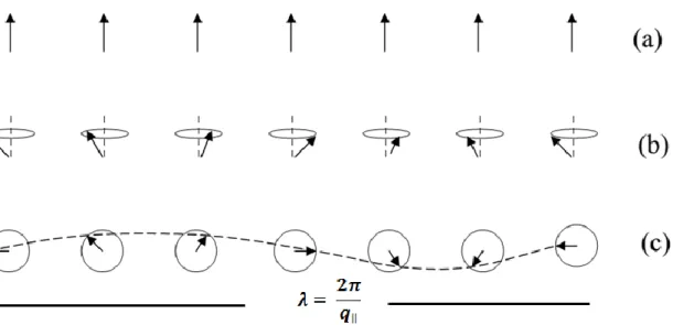
The semiclassical theory of the spin waves was further developed by Heller and Kramers [Hel34] in terms of precessing spins. Figure 2.16 shows the schematic view of spin wave in a ferromagnet. For a ferromagnetic material, there is interaction between neighboring
Figure 2.15: Semiclassical representation of spin wave in a ferromagnet: (a) the ground state (b) a spin wave of precessing spin vectors (viewed in perspective) and (c) the spin wave (viewed from above) showing a complete
38
electronic spins, which gives rise to a parallel alignment in the ground state (Fig. 2.15a). With perturbation, the spins will deviate slightly from their orientation in the ground state (Fig. 2.15b), and with this disturbance propagating with a wavelike behavior (Fig. 2.15c) through the material.
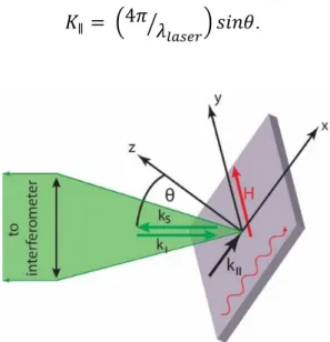
Spin waves with wave-vector (q) in the range 30 < q < 106 cm-1 are usually called dipolar magnetostatic spin waves or magnetostatic modes since it is almost entirely determined by magnetic dipole interaction. They were first reported by Damon and Eshbach [Dam61] in 1961. The frequency of the magnetostatic mode depends on the orientation of its wave-vector relative to that of the static magnetization due to the anisotropic properties of the magnetic dipole interaction. Spin waves with higher values of wave-vector, when the exchange interaction cannot be neglected, are called dipole- exchange spin waves.
Spin waves are the dynamic eigen-excitations of a magnetic system. They are used to describe the spatial and temporal evolution of the magnetization distribution of a magnetic medium under the general assumption that locally the length of the magnetization vector is constant. This is satisfied with if, first the temperature is far below the Curie temperature (Tc ); and
second, if no topological anomalies like vortices, are present. The latter is fulfilled for samples in a single domain state, i.e magnetized to saturation by an external bias magnetic field. Then the dynamics of the magnetization vector are described by the Landau-Lifshitz torque equation [Lax94]:
−1𝛾𝑑𝑴𝑑𝑡 = 𝑴 × 𝑯𝒆𝒇𝒇 (2.44)
where M = MS + m(R ,t) is the total magnetization, MS and m(R, t) are the vector of the
saturation and variable magnetization respectively, is the modulus of the gyromagnetic ratio for the electron spin (/2 = 2.8MHz/Oe). The effective magnetic field (Heff) is calculated as
variational derivative of the total energy function E:
𝑯𝒆𝒇𝒇 = −𝛿𝑴𝛿𝐸 = 𝑯𝒐+ 𝑯𝒅𝒆𝒎− (𝑀12) ∇𝐸𝑎𝑛𝑖+ (𝑀2𝐴
𝑆) ∇
2𝑴 (2.45)
where Ho is the applied magnetic field, Hdem the demagnetization field, Eani the anisotropy
energy, MS the saturation magnetization and A the exchange stiffness constant. All the
![Figure 3.1: Thin film deposition processes. Fig. is adopted from Ref. [Was12].](https://thumb-eu.123doks.com/thumbv2/9liborg/3123613.9100/42.892.124.731.689.1017/figure-film-deposition-processes-fig-adopted-ref-was.webp)