Vitaly Kaganov
A unified capital asset pricing model
Ujednolicony model wyceny aktywów kapitalowyh
Doctoral thesis
Supervisor: dr hab. Katarzyna Perez, associate prof. of PUEB
Department of Monetary Policy and Financial Markets Doctoral Seminars in English
Content
Spis treści ... 4
Introduction ... 5
Chapter 1. Theoretical background for capital asset pricing ... 9
1.1. History and idea of capital asset pricing ... 9
1.2. Normative theories of capital asset pricing ... 17
1.2.1. Expected utility theory of von Neuman and Morgenstern (1944) ... 22
1.2.2. Portfolio theory by Markowitz (1952) ... 27
1.2.3. CAPM ... 31
1.2.4. APT ... 37
1.3. Behavioral theories of capital asset pricing ... 43
1.3.1. Prospect theory of Kahneman and Tversky (1979) ... 49
1.3.2. Typical behavioral models ... 55
1.4. Comparison of normative and behavioral approaches to capital asset pricing ... 67
Chapter 2. Literature review on empirical tests of capital asset pricing ... 72
2.1. Tests of normative models ... 72
2.1.1. Tests of CAPM ... 72
2.1.2. Tests of APT ... 84
2.1.3. Fama and French three–factor model (1993) ... 92
2.1.4. Fama and French five–factor model (2015) ... 96
2.2. Tests of behavioral models ... 97
2.2.1. Testing typical behavioral models ... 98
2.2.2. Tests of sentiment proxies... 103
2.3. Tests of Technical Analysis ... 115
2.3.1. Historical context... 115
2.3.2. Technical trading tools and strategies ... 119
Chapter 3. Methodology and tests of unified capital asset pricing model ... 134
3.1. Fundamentals of the model ... 134
3.2. Methodology of the test ... 136
3.2.1. Definition of variables ... 138
3.2.2. Goals and hypotheses... 146
3.2.3. Analysis procedure ... 148
3.2.4. Data ... 152
3.3. Results of tests of the models ... 153
3.3.1. Results for the single models ... 153
3.3.2. Results for the models, derived from PCA ... 160
3.3.3. Comparison with normative and behavioral models ... 167
3.4. Conclusions ... 180 Final remarks ... 184 Reference ... 186 List of graphs ... 203 List of figures ... 203 List of tables ... 204 Annex ... 205 Summary ... 210
Spis treści
Wstęp ... 5
Rozdział 1. Podstawy teoretyczne wyceny aktywów kapitałowych ... 9
1.1. Geneza i istota wyceny aktywów kapitałowych ... 9
1.2. Teorie normatywne wyceny aktywów kapitałowych ... 17
1.2.1. Teoria oczekiwanej użyteczności von Neumana and Morgensterna (1944) ... 22
1.2.2. Teoria portfela Markowitza (1952) ... 27
1.2.3. CAPM ... 31
1.2.4. APT ... 37
1.3. Teorie behawioralne wyceny aktywów kapitałowych ... 43
1.3.1. Teoria perspektywy Kahnemana and Tversky’ego (1979) ... 49
1.3.2. Typowe modele behawioralne ... 55
1.4. Porównanie podejścia normatywnego i behawioralnego do wyceny aktywów kapitałowych ... 67
Rozdział 2. Przegląd literatury na temat testowania modeli wyceny aktywów kapitałowych ... 72
2.1. Testy modeli normatywnych ... 72
2.1.1. Testy CAPM ... 72
2.1.2. Testy APT ... 84
2.1.3. Trzyczynnikowy model Famy i Frencha (1993) ... 92
2.1.4. Pięcioczynnikowy model Famy i Frencha (2015) ... 96
2.2. Testy modeli behawioralnych ... 97
2.2.1. Testy typowych modeli ... 98
2.2.2. Testy mierników nastrojów rynkowych ... 103
2.3. Testy analizy technicznej ... 115
2.3.1. Kontekst historyczny ... 115
2.3.2. Narzędzia i strategie analizy technicznej ... 119
Rozdział 3. Metodyka i testowanie ujednoliconego modelu wyceny aktywów kapitałowych ... 134
3.1. Fundament modelu ... 134 3.2. Metodyka testowania ... 136 3.2.1. Definicje zmiennych ... 138 3.2.2. Cele i hipotezy ... 146 3.2.3. Procedura badawcza ... 148 3.2.4. Dane ... 152 3.3. Wyniki badawcze... 153
3.3.1. Wyniki dotyczące pojedynczych modeli ... 153
3.3.2. Wyniki modeli na podstawie PCA ... 160
3.3.3. Porównanie wyników z modeli normatywnych i behawioralnych ... 167
3.4. Wnioski końcowe ... 180 Zakończenie ... 184 Bibliografia ... 186 Spis wykresów ... 203 Spis schematów ... 203 Spis tabel ... 203 Aneks ... 205 Summary ... 210 Streszczenie ... 213
Introduction
In 1965 Fama (1965) established the Efficient Market Hypothesis (EMH) which main idea is to demonstrate that past information has no influence on the current price formation and the
random walk makes the prices unpredictable. The EMH argues that market prices (P) are
always on its fair value, i.e. it does not under/overpriced and equals the fundamental price (F): 𝑃 = 𝐹. Later, Shiller (1981) discovers large price fluctuations compared to the fundamental prices of the EMH theory, known as the volatility puzzle. Leaning on the Prospect
Theory of Kahneman and Tversky (1979), Shiller (1981) argues that the source of such
phenomenon lies in the non–rational human nature. Psychological or sociological background of an individual may motivate him/her to make non–rational decisions relatively to his/her investment, which prevents from an individual to reach the fundamental price, i.e. this implies that market observable price (P) does not equal the fundamental price (F): 𝑃 ≠ 𝐹.
Black (1986) argues that the reason for volatility phenomenon is some noise which exists all over the markets and creates a divergence from the fundamental value as a result of environmental circumstances, preventing normal distribution of information. Noise traders obtain lots of information, which comes out from technical analysts, economic consultants and stockbrokers, falsely believing this information is useful to predict the future prices of risky securities. Following Black (1986), it implies that market observable price (P) is the sum of fundamental price (F) and noise (N): 𝑃 = 𝐹 + 𝑁. In contrast, behavioral explanations and models are based on a specific psychological bias. Most common behavioral biases were generalized by Szyszka (2009) within his Generalized Behavioral Model (GBM). According to the model of Szyszka (2009), the market observable price (P) equals the sum of fundamental price (F) and behavioral component (B): 𝑃 = 𝐹 + 𝐵.
The main question, the literature tries to answer, is how investors react to new information, when 2 variants are possible ― rational–base reaction or behavioral reaction. It is also possible to understand that the deviation from the fundamental price is either noise or behavioral component, i.e. 𝑁 = 𝐵. Conducting the literature review, I suggest that all types of the investors are simultaneously present on the market. Hence, the market observable price (P) should be equal to the sum of fundamental price (F) and nonfundamental price (NF), which is sum of noise (N) and behavioral component (B):
𝑃 = 𝐹 + (𝑁 + 𝐵).
My suggestion has a potential to create a platform for one integrated and solid financial theory. I believe that integration of the best achievements from both theories will lead to better results and to more accurate financial reality description.
The main goal of my PhD thesis is to propose and to test a new approach which combines normative and behavioral approaches in one Unified Capital Asset Pricing Model. The creation of the unified model is motivated by unification of traditional and behavioral approaches that in turn leads to universality, where rational–based and behavioral–based investors use the same model to determine daily returns. From here the sub–goals are:
1. Presenting normative and behavioral approaches to asset pricing and comparing them. 2. Describing and comparing empirical findings on non–fundamental component as well as
on normative, behavioral and unified models.
3. Proposing and testing the mechanism allowing capital pricing assets, which can be used in investment decision process.
4. Comparing the proposed model to existing models and checking whether it has more predictive power than those models.
There are 3 hypotheses derived from these goals:
H1: Deviation components hypothesis ― the deviation from the fundamental price indeed can be explained in terms of noise and behavioral components, i.e. in terms of Technical
Analysis index and Sentiment Indicators.
H2: Explanatory performance hypothesis ― the Unified Capital Asset Pricing Model has a better explanatory power of the deviation from the fundamental price than traditional or behavioral approaches separately, which is expressed in higher 𝑅2. It is obtained when 𝑅2 ≥ 0.5 at least for the fully integrated regressions.
H3: Significance hypothesis ― the components of the Unified Capital Asset Pricing Model are statistically significant.
The methodology of this study is closely related to the existed literature with several modifications and applied within 4 stages and the data for 2 stock markets of the US and Israel in 2001–2017 is applied. At the 1st stage all the goals, hypotheses and variables are defined.
As the unified model assumes 3 powers are involved in the explaining daily returns, every single power accepts its unique measure. The fundamental returns are described by the CAPM
model for the Israeli market and by Fama–French five–factor model for the US market, which are determined by rational investors as the EMH suggests. The noise is expressed in terms of
Technical Analysis and the variables are evaluated according the methodology of Neely et al
(2014) with several modifications. The behavioral component is expressed by Sentiment
Indicators and evaluated according the methodology of Sadaqat and Batt (2016) and Yang and
Zhou (2015) also with several modifications, assuming it is determined by investors with psychological biases. The evaluation method for all models is the Principal Component Analysis (PCA) and estimation method is OLS. Both these methods are widely accepted in the literature. At the 2nd stage the ability of chosen technical and sentiment variables to explain daily
returns is examined and compared. The comparison is made among all relevant models (including three and fife-factor models) in both US and Israeli markets. At the 3rd stage analysis
technical, sentiment and unified predictors are created through the principal component. Further, explanation power with coefficient pattern and significance of all predictors for daily returns are compared. At the last, 4th stage, the integration of relevant fundamental
component with predictors, derived from PCA, is applied and further comparison between all the models is done. Moreover, in this stage hypothetical alternative model, where all the components are integrated directly after the PCA with the fundamental component, is presented and its results are compared to all other models. The analysis ends with the conclusions.
There are several points of this PhD thesis which are the contributions to the literature. Two different, sometimes contradicting theories exist side by side describing the same subject is a paradoxical situation. Probably if one theory could be better than the other, only one would survive. In my PhD thesis I introduce a Unified Capital Asset Pricing Model in order to fill the gap between normative and behavioral theories. The suggested model should answer the question whether it is possible to improve the performance of every single model separately by unifying both in one model. Theoretically, the unified model surpasses every single existed model in every possible parameter regarding the daily returns. Indeed, the findings demonstrate that unified model may contribute to explanation of both normative and behavioral approaches on the background of stable coefficients. In this situation the unified model improves the explanatory ability significantly in the US and Israeli markets. The integration of the fundamental factors leads to noticeable increase in the performance of all models in both markets. However, only the unified model has the most prominent
achievement. The value of 𝑅2 of the united model can easely exceed 0.5 and in vast majority of cases it exceeds 0.55 while for other models, including five–factor model, it hardly exceeds 0.5. Even in the case of the alternative model, where technical and sentiment predictors, retained from the principal component analysis, are directly integrated with fundamental factors into one model, the unified model still have a better performance. The unified model is able to improve explanatory power of the alternative model even more than those of the five–factor model regarding to the three–factor model.
In addition, it was found that all the models demonstrate similar coefficient patterns and predictive ability on the US and the Israeli markets, which may indicate that such phenomenon appears internationally. If so, the unified model is even more universal than it was assumed at the beginning. For this reason, such phenomenon deserves to be investigated deeper. The literature suggests to involve only 2 powers in the determination of returns. The unified model suggests 3 powers that include more types of investors what should describe the financial reality better than previous approaches. Indeed, it is found that unified model has the ability to improve the performance of the existed models significantly. The Unified Capital Asset Pricing Model is actually a first attempt to unify main financial theories into one solid platform. According to the results obtained in the study there is a high potential to achieve improvement in performance of existed models with subsequent creation of only one financial theory, describing the financial reality the most appropriate way.
The thesis contains of three chapters. Chapter 1 provides a theoretical background for different capital asset pricing theories/approaches, including leading models in each one of the fields. Chapter 2 contains most important and influential studies on the theoretical models that are introduced in Chapter 1. Chapter 3 provides full description and theoretical background of the proposed Unified Capital Asset Pricing Model, including tests and comparison of its results with those of existed theories and models.
Chapter 1
Theoretical background for capital asset pricing
1.1. History and idea of capital asset pricingThe question of saving financial resources remains vital in any era. Searching for the answer leads, in general, to two questions. First question is about the decision of how to save and the second is how to keep the actual purchasing power of the savings in the future. The future is uncertain, hence before the individuals raise a question of risks and subsequent loss of their savings. In order to reduce the negative influences of the risks, it is necessary to reduce the uncertainty or to perform a diversification or both. Predictability in some degree of confidence may reduce the uncertainty, hence many researchers try to develop sufficient models to forecast asset prices. Such models answer the question of future prices but also the question of the optimal saving spending.
In this chapter I present the fundamentals for the capital asset pricing theories and for the technical analysis. I concentrate on the historical and theoretical background as well as on the description of the main models for classical and behavioral approaches. At the end of the chapter the comparison between two main approaches is also done.
Capital Asset Pricing Theories
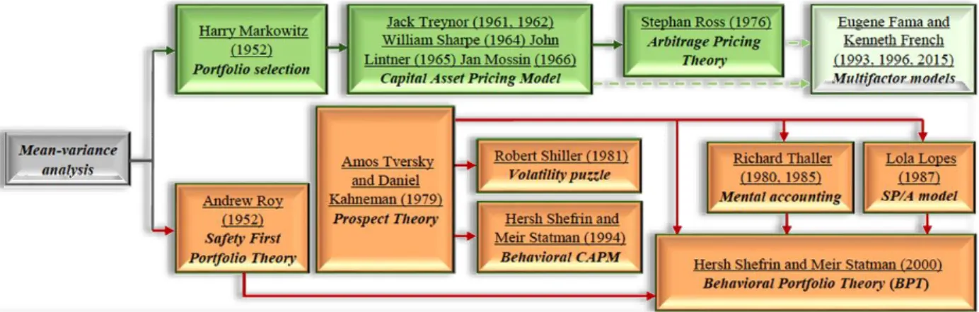
The modern capital asset pricing theories are based on mean–variance analysis as shown on Figure 1. Further evolution of those theories is divided on classical (normative) and behavioral finance.
Figure 1. Evolution of capital asset pricing theories
In 1952, Markowitz introduces a publication about the optimal portfolio choice, which is the Modern Portfolio Theory (MPT) based on a mean–variance analysis. The theory focuses on choosing an efficient strategy for risk diversification and justifies expediency of the diversification. The economic intuition behind the risk diversification is natural and understandable for individuals when the idea exists a very long time, but before Markowitz (1952) the diversification strategies were naive and made by a guess. He explains which assets are preferably included in a portfolio due to a perfect negative correlation with each other. In his work, Markowitz (1952) makes a connection between risk, measured in terms of volatility and returns. He also argues that it is possible to reduce the risks without any harm to the Rate of Return (ROR). He defines the set of points (portfolios) that are the most efficient due to their maximal diversification. The set creates a line of efficient frontier. Markowitz (1952) involves the risk–free asset assuming that combining a portfolio on the efficient frontier with the risk–free asset in a different proportion should give a better result than a portfolio which contains only risky assets. The MPT has a great contribution since it revolutionized the approach to finance as a whole, turning it to analytical. The MPT lays in the very foundation of further Capital Asset Pricing Model (CAPM) and of whole neoclassical capital asset pricing. The CAPM was independently and separately introduced by 4 researchers: Treynor (1961,
1962), Sharpe (1964) and Lintner (1965) as well as by Mossin (1966) and it is a straight logical
evolution of the Markowitz’ MPT. The main idea of the model is that the assets are correlated not only with each other but also with the market. Such correlation is the only factor that determines the expected returns, signed as 𝛽 coefficient, which plays a role of a risk premium. The CAPM takes the idea of Markowitz (1952) about measuring risks in terms of volatility further and argues that the market volatility is probably the risk, which should be compensated with an appropriate level of ROR through correlation with the market itself. If so, then the asset price that brings the risk–return pair to its optimal level is the equilibrium and called a fundamental price. The model is simple to intuitive understanding of every, even naive, investor that turned it to popular among both: the practitioners and the academia. The
CAPM is the first fundamental capital pricing model that is still in use even in present days.
The tests of the CAPM revealed that it does not fit to reality, which will be discussed in detail in Chapter 2. Ross (1976) fixes the misspoints of the CAPM and proposes a multifactor model, which is the Arbitrage Pricing Theory (APT). In this model, it is assumed that the correlation only with the market is insufficient since the market itself is depended on
macroeconomic environment. If so, there a specter of risks that influence the expected return where every one of them has its own correlation through its own beta coefficient.
In the parallel with Markowitz, Roy (1952) introduces another optimal portfolio preference. This publication becomes less popular than the MPT among the normative economists. Nevertheless, his work gave a push to behavioral finance and became known as Safety–First
Portfolio Theory (SFPT). Roy (1952) assumes that there is a probability that may cause an
overall collapse to an individual that he calls the probability of ruin. Such probability should be minimized that is equivalent to minimizing the number of standard deviations in which wealth level 𝑠 lies below the portfolio mean (𝜇𝑝) under normal distribution.
The difference of two theories lays in their motives. Markowitz (1952) keeps a place to an investor to decide about a desirable portfolio within the efficient frontier. Roy (1952) points the exact portfolio that an investor should chose and then constructs his CML. That is because Roy (1952) sees the world as a set of risks that some of them may cause total disaster to an individual. For this reason, an individual should prepare himself for such scenario by diversification among accessible assets and by choosing assets the manner that exceeds the probability of a disaster occurrence. This interesting interpretation of mean–variance analysis rose, as Roy (1952) believes, from unexplainable but observable behavior of individuals, driven by psychological aspects, though he is still leaning on an expected utility and normal distribution of portfolio returns as the normative theory suggests.
In 1979, Kahneman and Tversky introduce their Prospect Theory. They were interested to investigate how individuals make their decision facing the uncertainty and how they calculate a subjective probability to make their judgment of uncertainty comparable. For this reason, different prospects introduced to the participants and the results show that the individuals have a number of limitations. This real case study proves that the individuals have a different fundament for the uncertainty judgment than the one suggested by classical theory. It also shows how psychological biases may affect a way of how an individual makes his decision facing the uncertainty.
The theory describes a decision processes and tries to model real–life choices, rather than optimal decision as normative models do. According to the theory, the individuals make their decision leaning on the potential value of losses and gains with its respective probability rather than on the final real outcome.
and a new cluster of financial thinking, which is the behavioral finance, was created. This is the alternative approach to the classical normative theories raised as a result of the studies of the researchers like Shiller (1981) who observed volatility puzzle and explained it in the terms of investors’ non–rationality; Thaler (1980, 1985) who explained that money may have different value in an investor’s mind, which is known as mental accounting as well as Shefrin and Statman (1994) who made the behavioral extension to the CAPM. The heart of the
behavioral finance is the assumption that the human beings are not necessarily rational in the
sense of the traditional concept of Homo economicus. Therefore, individuals make their decisions involving non–economic factors.
Once the principals of the behavioral finance were established, the behaviorists turned to look after specific biases that may affect an individual’s investing behavior and cause a price to deviate from its fundamental value. Here every specific bias lay in a basis of a behavioral asset pricing model:
Barberis, Shleifer, and Vishny (1998) propose a model of investors’ sentiment;
Daniel, Hirshleifer, and Subrahmanyam (1998) assume the overconfidence of the investors;
Hong and Stein (1997, 1999) assume that the information distribution is gradual and hence is unequal.
Lopes (1987), based on the Prospect Theory, publicizes a decision–making model under
uncertainty, which is the SP/A model. She introduces a dual–sided problem that an individual should solve simultaneously. Lopes (1987) introduces a general individual descriptive problem, though she does not suggest any sufficient solution for it. According to the theory, an individual is about to solve how to secure himself from the subsequent fear additionally to achievement of aspiration from the subsequent hope. Possibly because of the fact that the problem should be resolved simultaneously, a solution was not introduced. The qualitative lesson from the SP/A model is that an individual should establish a portfolio in which he has a full control on the emotions of fear and hope, so that neither of them is dominant. Although, this intuition of dual choice problem is in the consideration of different behavioral researches under different definitions of the same variables.
The SP/A model, Prospect Theory and mental accounting with Roy’s safety–first model allowed Shefrin and Statman (2000) to develop the Behavioral Portfolio Theory (BPT) as a response to the MPT. In their model they propose that every single investor is not interesting
only in one investing portfolio, but he is likely to spread his investment between a number of portfolios, for each one its own goal and horizon. The model of Shefrin and Statman (2000) is a sort of the mean–variance analysis, looking towards the behavioral biases of the investors. The generalization of all psychologically biased models was made by Szyszka (2009). After a massive survey of behavioral literature (Szyszka, 2007), he realizes that only three psychological biases are widely common. For this reason, he decides to incorporate those three biases into a model, which is named Generalized Behavioral Model (GBM) today. The
GBM is successful in explaining many of the observed market anomalies.
Technical Analysis
Aside to the development of the fundamental theories, the literature discusses another approach of forecasting the direction and trend of the stock prices movement with different principles, which is the Technical Analysis (see Figure 2).
Figure 2. Technical Analysis development
Source: Own work
There is some evidence that several technical tools have been used to determine the stock prices already in the 17th century. The successful Jewish merchant from Cordoba, Jose de la
Vega (1688) wrote a book "Confusion of Confusions", which is the first book ever devoted to the stock market. In the book, he analyzes the prices behavior and introduces some techniques to forecast it. He describes Amsterdam Stock Exchange and different market tools like options of calls, puts and pools. In addition, he describes some speculative strategies. Another example of early Technical Analysis can be found in Japan. Munehisa Homma (1755) was the Japanese rice merchant who developed a unique trade technique that is in use even in the present days and known as the Candlesticks Charts. In his book, Homma (1755) claims that psychological aspects of the individuals are crucial. Emotional background composites the bear or the bull market. He notes that recognizing this can enable one to take
a position against the market.
In the western world, the technique was introduced by Nison (1991) that later claimed that the technique was actually created in 1800 and indeed was used on the Japanese rice market to forecast the prices. Candle is an abstract name for a figure that is created every trading day by open, close, daily high and daily low prices. Conditionally to the market forces a candle might be colored by black or white. Different forms of the following candles indicate some market positions that help a decision maker to "strike the market".
Though the existence of some old techniques of the Technical Analysis have been known since the 17th and 18th centuries, the main part of the theory development started in early
years of 20th century. Today it is Dow Theory after the name of the American journalist, co–
founder of Dow–Jones index and The Wall Street Journal. This theory was possible through the financial data accumulation in the hands of Dow. The theory with its 6 postulates, which is the basis for a decision making, was described in 1922 by the journal co–editors Hamilton, Rhea and Schaefer as a compilation of a momentum strategy. Those are:
(P1) – there are three types of trends: long (bullish/bearish);
medium swing that comes after the major movement;
short swing which represents the market reaction to a trend turn; (P2) – there are three phases to a market trend:
(1) first when the smart investors recognize the trend and buy/sell against the market;
(2) second when the trend becomes obvious and the active traders have started to buy/sell in large amounts, influencing the price;
(3) third when the whole market understands the trend and moves like it; (P3) – all the information is already priced;
(P4) – all the indices should be correlated with each other when a trend is changing through the timing may differ;
(P5) – a trend should be confirmed by a volume; (P6) – a trend is valid until a clear signal of its end.
Schabacker (2005), the editor for Forbes magazine and continuator of the work of Hamilton and Dow, concentrates in his book on a comparison between the fundamental indicators and
the technical ones. He also pays attention to the charts and patterns. He realizes that whatever a significant action appeared in the average, is a consequence of a similar action in some of the stock prices, making up the average. Schabacker was a pioneer of collecting, organizing, and systematizing the technical tools. He also introduced new technical indicators in the charts of stocks; indicators of a type that would ordinarily be absorbed or smothered in the averages, and hence, not visible or useful to Dow theorists (Edwards & Magee, 1948). The seminal work of the theory was done by the Schabacker’s nephew Edwards and Magee (1948). In their book "Technical Analysis of Stock Trends", they conduct the fundamental principles and the goals of the analysis. They revise the previous works in the area that are mostly concentrate on charts and trend recognition because of low computing power, and found it as good enough, but with their own extensions of new technical methods. They postulate only three principles:
(P1) – stock prices move in trends; (P2) – volumes go with the trends;
(P3) – a trend, once established, tends to continue in force.
The fundamentals of the analysis are as follows: all the relevant information is reflected in the prices and the past is a better indicator for the future, rather than external economic factors. The past reflects behavioral situations and how the individuals really reacted to it. If so, it is reasonable to assume that in similar situations the individuals will act the similar way as in the past. Technical Analysis believes that investors collectively repeat the behavior of the investors that preceded them, which allows predicting the prices behavior. The goal of the analysis is to identify, using the technical tools, a trend or a swing where all the market should move and by this way to earn an advantage before the market, i.e. to ride the trend. This is the main difference with the fundamental theories that try to determine a price.
The theory became demanded and popular again in late 80s and middle 90s of 20th century
with the evolution of computer technologies. Computers allowed the location of the important points in the charts and the analysis of the data much faster. Computer technologies helped to develop new analysis tools and techniques and new wave of publications swept the shelves in the forms of guides and manuals.
In the mid–90s, Technical Analysis pushed the idea of the Fractal Market Hypothesis (FMH) introduced by Peters (1991, 1994). Fractal is a functionally described geometric form that is a
replica of a larger same–form object, for example a tree or a leaf. This means that there is an object that contains smaller parts that geometrically have the same shape. In the sense of financial markets, a price changing, sometimes, repeats itself in a form of patterns that allows assuming like repeating is a natural price behavior.
First, it was discovered by Mandelbrot (1963) in 2 effects: Noah effect is the sudden discontinuous price changes and Joseph effect when a price can stand for a short period yet suddenly change afterwards. Both effects violate the assumption of assets’ prices normal distribution. To describe his results, Mandelbrot (1963) uses the Chaos Theory.
The Chaos Theory is crucial for understanding the FMH. Though first attempts of Poincare (1892, 1893, 1899) to analyze mathematically the behavior of the dynamical systems, it was Lorenz (1963) that pioneers and develops the idea. Lorenz (1963) accidentally found that some systems are extremely sensitive to initial conditions. A miserable change in very short–terms may lead to significant changes in long–terms, making the dynamics mostly unpredictable. He begins to investigate the phenomenon and concludes that such system looks chaotic at first glance, but stem under some functionally described order. The chaotic functions are complicated for solving and the mathematics behind the Chaos Theory is not fully understood. The theory tries to build a testable environment and uses complexed mathematics to support the hypothesis. The FMH believes that with additional development of the chaotic mathematics, the prices can be exactly predictable. It is established on three assumptions:
(A1) The investors can be rational or irrational in their decisions. What is more important, the investors are deviated in 2 groups depending on their investing horizon:
the group of short–terms investors; the group of long–terms investors;
when an investment horizon is defined as the amount of time one plans to hold his money as an investment. In a case when the investors swing their strategy (becomes only one investors group), the market may crash by losing its liquidity. When another group is missing, no trading is possible;
(A2) The prices change on a basis of information that is relevant and meaningful to a certain investors’ group. Therefore, an equilibrium price does not exist because investors value their investments differently and existence of the irrational investors automatically drives prices out from its fundamental value;
(A3) The FMH believes that there is short–terms stochastic process but long–terms deterministic process.
Even though the Technical Analysis is popular among investors, it suffers from hard criticism. The normative theories cannot accept the Technical Analysis despite some similarity of its views, because the basis is fundamentally different. The question of the predictability for the normativists is still open and has a different origin. The past cannot predict the future, even if some connection may be found it is not obvious that the behavior may be repeated. There is no hard proof that the Technical Analysis works in the mathematical or statistical sense. The main criticism is around the testability of the patterns.
1.2. Normative theories of capital asset pricing
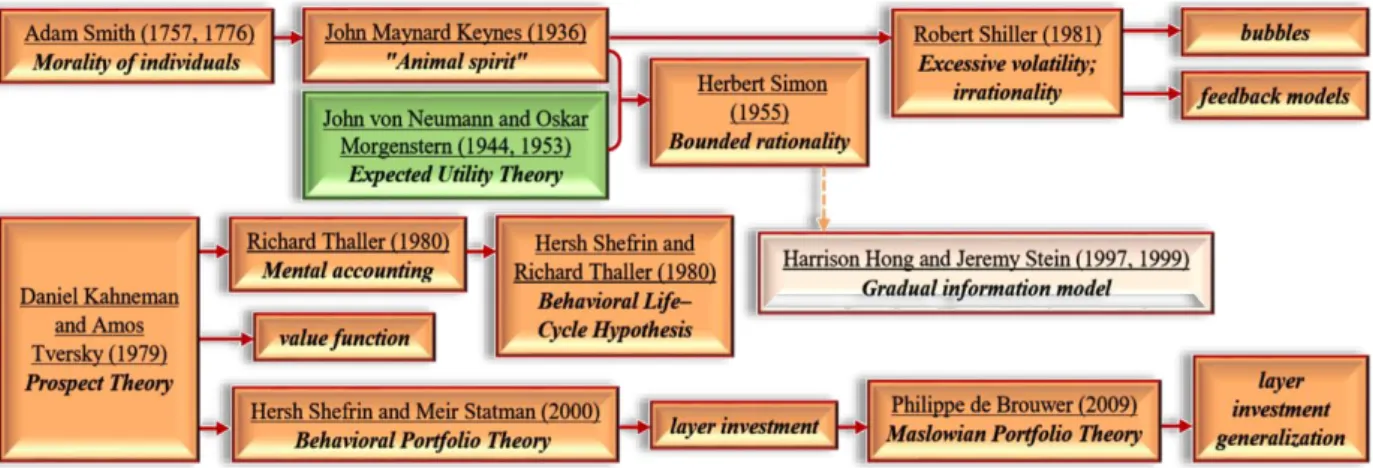
The roots of normative theories of capital assets pricing are in the foundation of economics as a science itself (see Figure 3). Smith (1757, 1776) and his contemporaries describe the philosophical aspects of the concepts for liberal economics that became familiar with classical
economics. In his books, Smith (1757, 1776) formulates the academic thoughts of his era.
Some of them were progressively new and some were paraphrasing or extending exiting principles. In his famous books "The Theory of Moral Sentiments" (1757) and "An Inquiry into the Nature and Causes of the Wealth of Nations" (1776) (or simply "The Wealth of Nations"), he discusses the topic of free economics and proposes some postulates of new principals. Even in the present days some of Smith’s principles are still valid.
Figure 3. Background for normative theories
Source: Own work
In particular, Adam Smith adopts the term of laissez faire from the exiting in his days understanding of the economics and further develops it. He uses a term of invisible hand ― an ability of a market to regulate itself by the inner power that comes out from the behavior
of the individuals. The individuals intuitively understand the market mechanisms and they compose the market in such way, allowing them to reach equilibrium ― a special condition where all parts of the market are balanced.
Smith (1757, 1776) postulates that all individuals should be driven by their own egoism. Egoism dictates the best for an individual and if all individuals may obtain their best, the overall social wealth should reach its maximum and hence desirable level. At this level, minimal poorness can be reached and will be necessary to obtain if an egoistic individual is free to act. A struggle of the individuals in the free market to obtain their possible maximum wealth should bring the individuals to a self–interested competition that would tend to benefit society as a whole by keeping prices low, while still building in an incentive for a wide variety of goods and services. As well as the individuals maximize their wealth, as Smith (1757, 1776) argues, the firms maximize their profit. He assumes that such concept is right relatively to both: an individual as a single unit or a whole nation as a single organism (in the sense of micro/macroeconomics).
In order to make this economic model to work, first, an economic agent must be defined. However, the egoism is not the only power that motivates the individuals, it is also the happiness. Smith (1757, 1776) describes the agents as rational individuals. Rationality, the fundamental term of all normative theories, is a specific behavior where an individual has some inner consistent clear and complete preference system, allowing him to rate all the products relatively to its usefulness that may be described by a utility function as a mathematical expression. An individual should prefer more than less and he prefers to enjoy than to suffer but to have less loss then more in reverse look. A rational man is motivated by facts and reasons to act and chooses to perform the action with the optimal expected outcome. Emotions are not rational and hence, are not taken into account during economic decisions of the individuals, because if they are, the optimal decision cannot be reached. Later, in the 19th century, Mill (1836) extends the definition of rationality based on the
Smith’s concept and defines a term of Homo economicus. Homo economicus is a consistently rational, self–interested and labor–averse individual. The goals of such man are very specific and predetermined while he seeks to obtain it in greatest extent with the minimal possible costs. This definition is in use as approximation of Homo Sapiens and allows modeling economic behavior of human.
normative mathematical analytical tools. All this created a neoclassical economical approach which is recognized today as a mainstream school. The neoclassical economists postulate three principles that are the fundament of all in the economy. They are as follows:
(P1) – people have clear and complete preference system between outcomes that can be measured and translated to a value; the values have been produced with a utility function and comparable;
(P2) – all individuals maximize their wealth and all firms maximize their profits;
(P3) – the individuals make their decision according to expected utility and full and relevant information.
Neoclassical economists believe that the rationality rules all over and the individuals have accesses to all relevant information that is the very center of their decision. If so, it is reasonable to assume that formation of demand and supply has to be created with the same principles and talking about a stock market, the information is already priced within the stocks. First determination of stock prices variability was made by Regnault in 1863. He argues that the stock prices evolve according to a random walk and hence, are unpredictable. He was the first who used statistics and probabilities to determine the stock prices. Further popularization of the idea of random prices movements refers to Kendall (1953). The theory states that stock price fluctuations are independent of each other and have the same probability distribution, but that over a period of time, prices maintain an upward trend. Past movement or direction of the price of a stock or overall market cannot be used to predict its future movement. In 1965, in his doctoral thesis, Fama introduces the Efficient Market Hypothesis (EMH) based on the neoclassical principles. The EMH considers the agents as super rational individuals that have full accesses to all possible relevant information and properly use it in an extremely short time, where a rational agent is the one who wishes to maximize his expected return for a given level of risk. Subsequently, all the news are rapidly and fully reflected in the investment prices as it become known. Due to a short time pricing, competition drives all the information into the price quickly and there is no possibility to make any profit from the information in the long–run terms. This means that the assets are always traded on their fair
value, i.e. they are not under/overpriced.
The available information is divided into 2 types:
will reflect beliefs of the market before the event actually occurs;
– the other type is all available information, which includes past information, current
information, and announcements of future events.
The market price is not required to shift instantaneously or adjust to the perfect price following the release of new information. After an announcement is released, the price only must change quickly to an ''unbiased estimate of the final equilibrium price". The final equilibrium price will be reached after investors decide the new information’s relevance on the stock price.
There are three forms of the EMH: weak, semi–strong and strong.
– The weak form describes a situation where all available past and historical information
is already priced by the market and is reflected in the stock prices. If so, the past information has no influence on future prices, hence, it is impossible to make any excessive returns in the future leaning on the historical data and knowledge. This means that any Technical Analysis tool is useless. Future price movements are determined exclusively by the information which is not contained in the price series. Therefore, the prices changes must follow a random walk and consequently, must be unpredictable. Although, the insiders that hold information before it is released to the market may obtain some abnormal returns above the average for a very short period.
– The semi–strong form describes a situation where new public available information is
rapidly incorporated into the stock price. This implies that an investor cannot act on new public information and expect to earn any excessive returns. This time, neither the technical nor the fundamental analyses are able to produce any excessively returns above the predicted average.
– The strong form describes a situation where the stock prices fully reflect all public or
nonpublic information, which means that even insiders cannot make abnormal profits in the market. The information about future events is also properly priced.
The EMH implies that no individual can benefit from the market consistently because stock prices follow a random walk and cannot be anticipated or be a basis for extra profit. If someone does outperform the market, it is only through luck or by a statistical chance. This means that a portfolio manager will not succeed to compose a better portfolio then those that were created by a blind random selection. The answer lies not in the returns of the chosen stocks, but in the risk of the chosen portfolio. If the market is efficient, portfolio managers are
still able to obtain the appropriate level of diversification of the portfolio, they are able to obtain a higher return for a given risk level. This should eliminate firm specific risk and leave the portfolio only with systematic risk.
Also, it is important to understand that the EMH, assuming investors rationality, does not exclude the existence of non–rational individuals. Their activity may be seen as distortion of a pricing process that may create a disparity in the prices. As the theory suggests, due to prominent majority of the rational investors, such disparity will be closed quickly because rational investors are able to recognize it and act to obtain an extra profit until complete disparity closing.
The underlying principal of the EMH is established through the Central Limit Theorem (CLT). The CLT states that as sample independent random variables are approaching infinity, the probability function is approaching the normal distribution curve. From this concept, the EMH assumes that market changes are random and if the market changes are plotted over a period of time they should construct the normal distribution curve. This way the CLT can be applied to historical data in order to find a correlation between the EMH and the observed financial market from which the data is taken.
Samuelson (1965) publishes a proof of prices random–walk behavior if a market holds the
EMH, which is acceptable theoretical support of the theory of Fama (1965). Further, Fama
(1970) publishes a review of both the theory and the empirical evidence for the EMH. His paper claims that the stock market holds the micro efficiency, but not the macro efficiency. Samuelson (1998) was sharing such opinion arguing the EMH is more suitable with individual stocks rather than with the aggregate stock market. Additional strong support of the random walk is issued by Malkiel (1973) in his influential book "A Random Walk Down Wall Street". The EMH describes a capital market structure in the manner of normative vision and successfully integrated into existed normative approaches. Behind almost every normative capital asset pricing model stands the assumption that the EMH is valid. The CAPM, APT and further extensions of the CAPM, like Merton’s (1973) ICAPM, accept the EMH as a starting point. Today, the concept of the EMH and its assumptions provide a solid platform and paradigm for modern normative economists.
In the following parts, next important and fundamental theories will be discussed:
Expected Utility Theory (EUT) of von Neuman and Morgenstern (1944, 1953), which is a normative basis for decision making process under uncertainty.
Modern Portfolio Theory (MPT) of Markowitz (1952), which is the normative basis for optimal investing choice.
Capital Asset Pricing Market (CAPM) of Treynor (1961, 1962), Sharpe (1964), Lintner (1965) and Mossin (1966), which is the normative equilibrium of the capital markets and the first fundamental model of asset pricing as a whole. Several popular extensions for the model will be also introduced.
Arbitrage Pricing Theory (APT), which is the multifactor version of the CAPM and the second fundamental pricing model, including several extensions.
1.2.1. Expected utility theory of von Neuman and Morgenstern (1944)
Financial decision making under uncertainty is a regular activity of every individual. People cannot predict the future but also cannot avoid facing the future decisions. It is more likely that people build their financial strategies according to some possible expected outcomes. Figure 4 shows the theoretical background for decision making process which leads to the expected utility theory of von Neuman and Morgenstern ― a basis for modern capital asset pricing models.
Figure 4. Background for utility theory of von Neuman and Morgenstern
Source: Own work
The first definition for decision making system under uncertainty was made by Daniel Bernoulli (1738). He tries to resolve the St. Petersburg paradox for infinite expected utility that was introduced by his cousin, Nicolas Bernoulli in 1713. Particular, he uses a coin toss game to demonstrate the limitation of expected value as a normative decision rule. Bernoulli’s analysis of the dynamics of the St. Petersburg paradox leads him to appreciate that the subjective value, or utility, that an outcome has is not always directly related to the absolute
amount of the payoff or its expected value. Out of his analysis, he proposes a utility function to explain a choice behavior of the individuals.
Bernoulli (1738) proposes and applies a concave form for a utility function and uses a logarithmic function of 𝑈(𝑥) = 𝑙𝑛(𝑥) to represent it. He analyzes such function in order to measure the risks and he realizes that an individual care about the expected utility of possible outcomes rather than about the outcomes themselves. The concave function form allowed him to represent 2 important parameters:
(1) the risk aversion of a person ― he makes effort to avoid the risks, when for every agent, it is possible to apply different utility function with different degree of own risk aversion; (2) the risk premium ― dissonance between an individual’s utility and taking a part in a
gambling.
Indirectly, he means that a decision should be made on a basis of a marginal utility of money, i.e. subjective money value may vary from person to person. In addition, he makes a connection between expected value to its probability, where the risk premium should be higher for events with low probability and vice versa.
In 1789, Bentham publishes a book devoted to the utility issue. There he uses an increasing function to describe the greater happiness or utility from enjoying consuming greater quantities of a divisible good and he argues that the function should be concave due to diminishing marginal utility. Later, it was found that any function that is affine transformation of a given utility function would keep the same characteristics as the original given function. In other words, linear transformation would not harm the initial function. All the family of functions that hold such transformation is called cardinal functions and all concave functions that are similar to logarithmic functions are called Bernoulli functions.
Cardinal utility approach was proposed by Marshall (1890). He uses it to explain demand curves and the principles of substitution. Marshall (1890) assumes that the utility of each commodity is measurable and the most convenient measure is money. Hence, marginal utility of money should be constant. He also argues that if the stock of commodities increases with the consumption, each additional stock or unit of the commodity gives him less and less satisfaction. It means that utility increases at a decreasing rate. Additionally, he assumes that utilities of goods are independent, where utility obtained from one commodity is not dependent on utility obtained from another commodity, i.e. it is not affected by the
consumption of other commodities.
In early 20th century the economists such as Allen and Hicks (1934) and Samuelson (1938)
successfully campaigned against notions of cardinal utility, mainly on the grounds that the postulated functions lacked measurability, parsimony, and generality compared to ordinal measures of utility.
Contrary to the notion of cardinal utility formulated by neoclassical economists who hold that utility is measurable and can be expressed numerically or cardinally, ordinalists state that it is not possible for consumers to express the satisfaction derived from a commodity in absolute or numerical terms. Ordinal measurement of utility is qualitative but not quantitative, where the preference is made by ranking the goods. Allen and Hicks (1934) argue that cardinal utility is less realistic because of its inability of quantitative measurement. Cardinal approach supposes that if a preference can be expressed by a utility function the optimal choice should be based on utility marginal measurement. Contrary, ordinal approach supposes that a choice is a result of comparing between different indifference curves.
Indifference curve is defined as a set of points on the graph, where each is representing a
different combination of two substitute goods, which yield the same utility and give the same level of satisfaction to a consumer. Such curves are orderly arranged in a so–called indifference
map where none of the curves crosses the other. Two conditions are necessary for existence
of ordinal utility function: those are completeness and transitivity. The ordinal utility concept plays a significant role in consumer behavior analysis. Modern economists also believe that the concept of ordinal utility meets the theoretical requirements of consumer behavior analysis even when no cardinal measure of utility is available.
At the middle of the 20th century, just as the ordinalists’ victory seemed complete, a small
group of theorists including von Neumann and Morgenstern1 (1944, 1953) build a new
foundation for the cardinal utility. Von Neumann and Morgenstern turn the Bernoulli’s model assumptions upside down and use preferences to derive utility.
They prove that if a decision maker’s risky choices satisfy a short list of 5 plausible consistency axioms, then there exists a particular utility Bernoulli function whose expectation maximize those choices. Also, they conduct that only if an individual is rational, his utility
function will hold the necessary axioms. The axioms were introduced in their publication of
1 Von Neumann, J., & Morgenstern, O. (1944, 1953). Theory of Games and Economic Behavior (2nd ed.).
1947 and as von Neumann and Morgenstern believed, they should be simple, clear and intuitively understandable. The axioms are:
– Completeness: This axiom ensures that for every possible choice, an individual is able
to choose between them. A rational individual has an ability to rank all the choices and he will prefer the one that gives him maximum utility. For every new choice, an agent may compare it with the existed and still be able to make a choice. The formal definition is given as follows: For every two lotteries, 𝐿1and𝐿2, one should be hold, or
𝐿1 ≺ 𝐿2 or 𝐿1 ≻ 𝐿2 or𝐿1~𝐿2, which is either 𝐿1is preferred, 𝐿2 is preferred, or the
individual is indifferent between𝐿1and𝐿2.
– Transitivity: This axiom ensures a choice consistency that is correct for every rational
individual. Existing preference cannot be changed and for all possible choices, the most preferred one over others is still be preferred all the time. The formal definition is given as follows: For every three given lotteries, when𝐿1 ≾ 𝐿2 and 𝐿2 ≾ 𝐿3 it has to hold
that𝐿1 ≾ 𝐿3.
– Continuity: Such axiom ensures that for any gamble, there exists some probability such
that an individual is indifferent between the best and the worst outcome. Mathematically, this axiom states that the upper and lower contour sets of a preference relation over lotteries are closed. This axiom is actually a particular case of the Archimedean property that says that any separation in preference can be maintained under a sufficiently small deviation in probabilities. The formal definition is given as follows: For every three given lotteries, when𝐿1 ≾ 𝐿2 ≾ 𝐿3 there is a
probability of 𝑝 ∈ [0,1] such that𝑝𝐿1+ (1 − 𝑝)𝐿3~𝐿2.
– Monotonicity: This axiom ensures that a gamble which assigns a higher probability to
a preferred outcome will be preferred to one which assigns a lower probability to a preferred outcome, as long as the other outcomes in the gambles remain unchanged.
– Independence of irrelevant alternativesor substitution: Such axiom ensures that
given a preference of one lottery to another, adding the same lottery to the previous should not change the existing preference. Rational individual should concentrate only on those parts that are needed to be compared and to make his choice only with relevant parts. This axiom allows to reduce compound lotteries to simple lotteries. The formal definition is given as follows: For every two given lotteries, when𝐿1 ≺ 𝐿2 then
After defining the axioms, it is possible to introduce the idea of expected utility function that also holds the linear transformation. Von Neumann and Morgenstern (1944, 1953) define that if the axioms hold, then it is possible to adjust an expected utility function to a rational individual, which is linear in its probabilities, called Von Neumann–Morgenstern (vNM) function and given as follows: A utility function 𝑈: 𝑃 → 𝑅 has an expected utility form (the
vNM) if there are numbers (𝑢1, … … , 𝑢𝑛) for each of the 𝑁 outcomes (𝑥1, … … , 𝑥𝑛) such that
for every𝑝 ∈ 𝑃,𝑈(𝑝) = ∑𝑛𝑖=1𝑝𝑖𝑢𝑖. This implies that:
𝐸(𝑈(𝑥)) = 𝑝1𝑈(𝑥1) + ⋯ + 𝑝𝑛𝑈(𝑥𝑛). (1.1) If individual’s preferences can be represented by expected utility function then the linearity of expected utility means that his indifference curves must be parallel straight lines. The same linearity property also implies that the indifference curves must be parallel and vice versa. So that given the other axioms, the independence axiom is also equivalent to having indifference curves that are parallel straight lines and hence equivalent to having preferences that are representable by a vNM expected utility function.
The vNM Expected Utility Theory (EUT) was applied to normative economies, especially in the game theory, but it has a number of limitations. Assuming individuals’ rationality in theory, however in practice, the individuals may do not always behave rationally in the sense of vNM. In 1953, Allais designs a choice problem known as Allais paradox to show an inconsistency of actual observed choices with the predictions of the EUT. He presents his paradox as a counterexample to the postulate that choices are independent of irrelevant alternatives, i.e.
substitution axiom, which is the most prominent example for behavioral inconsistencies
related to the vNM axiomatic model of a choice under uncertainty. The paradox shows that an individual, being rational, prefers not to achieve the maximum expected utility but to achieve absolute reliability.
The empirical evidence on the individual’s choice shows that the individuals systematically violate the EUT. To response to these findings, several modifications were introduced, mostly by weakening the vNM axioms. They include weighted–utility theory by Chew (1983); implicit
expected utility by Dekel (1986) and Chew (1989); regret theory of Bell (1982) as well as rank– dependent utility theories by Quiggin (1982), Segal (1987, 1989) and Yaari (1987). All of those
theories are normative and only the Prospect Theory has non–normative basis in attempt to capture individual’s attitudes to risky gambles as parsimoniously as possible.
1.2.2. Portfolio theory by Markowitz (1952)
The idea of risk diversification is very old. The bible and the Talmud contain advises, how to divide the investment to avoid the risks. Individuals intuitively understand that holding all their savings in one form of investment could be dangerous, though they do not know what disaster may happen. However, advice of a strategy for risk diversification may be good but does not mean it is efficient. Choosing a portfolio of assets in the stock market is not so trivial. The question of portfolio choice efficiency was very crucial for Markowitz (1952)2. The work of Markowitz (1952) really has changed a vision of what the stock market was, in the sense of optimal risk adjustment. It was not a guess concept any more, but a true financial market analysis. Today, the method of Markowitz (1952) is known as the Modern Portfolio Theory
(MPT) and is recognized as mean–variance analysis.
A process of choosing an optimal portfolio contains 2 stages:
– The first stage starts with an observation as well as experience and ends with beliefs
about the future performance of available assets.
– The second stage starts with the relevant beliefs about the future performance and
ends with the choice of a portfolio3.
It is true that an investor attempts to maximize discounted value of future returns. Since the future is uncertain, those values should be replaced with expected returns4. Due to price
fluctuations, the returns, even expected, may vary. The higher the magnitude, the greater the risk that the desirable expected return will be missed. For this reason, Markowitz (1952) measures the risk as a variance of deviation from some expected average which is expressed in terms of standard deviation5.
Given 𝑁 securities, the concept of expected return for any portfolio is expressed as follows:
𝑅 = ∑ ∑ 𝑟𝑖𝑡𝑑𝑖𝑡 𝑁 𝑖=1 𝑋𝑖 = ∞ 𝑡=1 ∑ 𝑋𝑖 𝑁 𝑖=1 (∑ 𝑟𝑖𝑡𝑑𝑖𝑡 ∞ 𝑡=1 ) → 𝑅 = ∑ 𝑋𝑖𝑅𝑖, where:
2 Some studies were done before Markowitz (1952) in this direction. For example, Hicks (1935) involves risk
measure in his analysis; Marschak (1938), the Markowitz’ supervisor, used the means and covariance between goods as utility approximation; Williams (1938), Cowles (1939) and Leavens (1945) who illustrated the benefits of diversification based on the assumption that risks are independent.
3 Markowitz, H.M. (Ed.). (2008). Harry Markowitz: Selected works. World Scientific ― Nobel Laureate Series, 1:
World Scientific Publishing Co. Pte. https://doi.org/10.1142/6967.
𝑟𝑖𝑡 – the expected return rate at time 𝑡 of security𝑖;
𝑑𝑖𝑡 – the discount rate;
𝑋𝑖 – the amount of money spent in𝑖;
𝑅𝑖 – the discounted return and independent of𝑋𝑖.
Therefore,𝑅 is the weighted average of 𝑅𝑖 with non–negative weights of𝑋𝑖, hence 𝑅
should be maximized. Returns are random variables, i.e. its value is generated by a chance. The proportions of the assets in a portfolio are decided and fixed by an investor. In this case, two variables are to be determined: the expected return which is given by:
𝐸(𝑅) = ∑ 𝑋𝑖𝜇𝑖 𝑛
𝑖=1
and its variance, given by:
𝑉(𝑅) = ∑ ∑ 𝑋𝑖𝑋𝑗𝜎𝑖𝑗 𝑛 𝑗=𝑖 𝑛 𝑖=1 , where: ∑ 𝑋𝑖 𝑛 𝑖=𝑖 = 1.
Another important decision factor for better assets combining is the correlation between the chosen assets which is expressed by the covariance 𝜎𝑖𝑗 = 𝜌𝑖𝑗𝜎𝑖𝜎𝑗. When the covariance
coefficient 𝜌 is equal to 1, perfect correlation occurs and this is the worst scenario for an investor. The covariance measures diversification when the best diversification is obtained with uncorrelated assets, i.e. the covariance coefficient 𝜌 is equal to (–1). Before this method,
simple or naive diversification took place. The investors intuitively understood the advantages
of such action but no measurement or criterion existed. Markowitz (1952) makes three main assumptions:
(A1) – selling in short position is impossible. This ensures that all weights of chosen assets in a portfolio will be non–negative, hence the sum of all the weights equals to 1; (A2) – all the individuals are risk averted. This is behavioral definition of individual’s choice
(with underlying rationality assumption);
(or standard deviation) and represents risk; or maximize the expected return in a given level of variance.
According to the assumptions, Markowitz (1952) constructs an ellipsoidal line that contains all mean–variance efficient portfolios set, called the efficient frontier (though Markowitz himself did not call it that way), which is given by minimizing the following equation:
𝑋𝑇𝛴𝑋 − 𝑞𝑅𝑇𝑋, (1.2)
where:
𝑋 – a vector of portfolio weights with the sum of all weights is equal to 1; 𝛴 – the covariance matrix between the returns of the assets in the portfolio; 𝑞 – a non–negative risk tolerance factor;
𝑅𝑇𝜔 – the expected return on the portfolio.
All over the efficient frontier it is possible to obtain a higher ROR, in a given level of standard deviation. As Markowitz (1952) suggests, an investor should make his portfolio choosing with regard to the efficient frontier.
However, none of the whole ellipsoidal line is appropriate for the portfolio choosing. Among all possible mean–variance efficient options only the optimal portfolios are acceptable which are located on the grey part of the ellipsoidal line as shown in the Graph 1.
Graph 1. The efficient frontier and the optimal portfolios set
Source: Own work
For Markowitz the efficiency was not the only problem. Additionally, he was looking for the σ
𝑚𝑖𝑛{𝜎2− 𝐴𝜇}, where A is a degree of personal and unique risk aversion. When risk–free
lending and borrowing is possible with zero variance and return r, then the combination of a portfolio with riskless asset may improve the diversification. In this case, the expected return may be written as:
𝐸(𝑅) = 𝑟 +𝜇𝑝− 𝑟
𝜎𝑝 𝜎. (1.3)
Here, maximizing the expected return for a fixed level of risk is equal to maximizing its slope and the optimization problem accepts the next form:
𝑚𝑎 𝑥 {𝜇𝑝− 𝑟 𝜎𝑝 }, 𝑆𝑢𝑏𝑗𝑒𝑐𝑡𝑡𝑜 𝑉(𝑅) = ∑ ∑ 𝑋𝑖𝑋𝑗𝜎𝑖𝑗 𝑛 𝑗=𝑖 𝑛 𝑖=1 , ∑ 𝑋𝑖 𝑛 𝑖=𝑖 = 1.
A portfolio giving 𝜇𝑝 and 𝜎𝑝 that maximizes the slope is called Optimal Portfolio of Risky Assets (OPRA). Giving a risk–free asset, OPRA is a portfolio on the efficient frontier that is
connected with a line to a risk–free asset, as shown in the Graph 2. Such line reflects all optimal weighted portfolios within a given risk level and a risk–free asset. This line is called Capital
Asset Location (CAL) and Markowitz’s suggestion is choosing a portfolio within the CAL.
Graph 2. The Capital Asset Location (CAL) line and the Optimal Portfolio of Risky Assets (OPRA)
Source: Own work
σ µ 𝑟1 𝑂𝑃𝑅𝐴1 𝐶𝐴𝐿1
Despite a great contribution of the MPT to the theoretical and mathematical understanding of a stock market, a number of criticisms is addressed to Markowitz (1952). The first criticism is concentrated on the lack of parameters to determine an optimal portfolio. Many necessary macroeconomic factors, such as inflation, income, etc., are not involved in the process and nor the fundamental analysis as Graham and Dodd (1934) suggested.
Additional strong criticism refers to a doubt whether a volatility is a good measure of a risk. Standard deviation, as a symmetric estimator, measures the upside movements as equally bad as the downside movements. Obviously, for an investor upside movement is desirable but the downside movement should represent a real risk exposure. Sometimes, downside movement could be viewed differ if before, an investor won upside movement. Post–Modern Portfolio
Theory (PMPT) uses downside risk of returns which is based on the Markowitz’ (1959) semi–
variance instead of the mean–variance to resolve the problem (see Estrada (2002, 2007)). Finally, speculative stocks which are extremely volatile do not fit into this format as they certainly do not give superior returns, as a diversified group or otherwise.
Another problem refers to the assumption of returns distribution that is supposed to be normal and symmetric. In the reality, the stock returns not always follow a normal distribution. There is a considerable evidence of skewness, fat tails, kurtosis etc. The volatility cannot reasonably be predicted from a normal distribution. Mandelbrot (1963) and Fama (1965) are the first who emphasize that the stock returns are not following the Gaussian distribution. Further early studies, including Officer (1972), Clark (1973), McCulloch (1985) and Bollerslev (1987), demonstrate that the assumption of returns normal distribution may be insufficient.
1.2.3. CAPM
The CAPM is the central fundamental model, which has conquered the academia for decades. Despite the fact that today the investors relay less on the model, it pushed the development of other important normative models (see Figure 5).
The Capital Asset Pricing Model (CAPM), introduced separately by Treynor (1961, 1962),
Sharpe (1964), Lintner (1965) and Mossin (1966), is the logical evolution of the Markowitz’s
(1952) MPT. Hence, a strong connection and similarity between the CAPM and the MPT are present. The goal of the model is to determine a required rate of return to justify adding an asset to an already well–diversified portfolio. Another proposal of the model is a determination of compensation for bearing extra risks above the risk–free rate contrary to the