TRENDS
in
Sport Sciences
2014; 4(21): 195-206. ISSN 2299-9590The main aim of this paper is to provide some practical guidance to researchers on how statistical power analysis can be used to estimate sample size in empirical design. The paper describes the key assumptions underlying statistical power analysis and illustrates through several examples how to determine the appropriate sample size. The examples use hypotheses often tested in sport sciences and verified with popular statistical tests including the independent-samples t-test, one-way and two-way analysis of variance (ANOVA), correlation analysis, and regression analysis. Commonly used statistical packages allow researchers to determine appropriate sample size for hypothesis testing situations listed above.
KEYWORDS: power analysis, hypothesis testing, sample size estimation, sport science, examples.
Received: 15 September 2014 Accepted: 17 October 2014
Corresponding author: maciejtomczak5@gmail.com
1University School of Physical Education in Poznań,
Department of Psychology, Poznań, Poland
2Adam Mickiewicz University in Poznań, Faculty of English,
Poznań, Poland
3Adam Mickiewicz University in Poznań, Institute of
Psychology, Department of Foundations of Psychological Research, Poznań, Poland
What is already known on this topic?
The power of a test is the probability of correctly rejecting the null hypothesis. In a practical sense, the power tells us how likely we are to detect a statistically significant effect in our data (e.g., a difference between two groups, or a correlation), given that it really exists in the population. Taking the power of a test into account, appropriate sample size may be estimated already at the planning stage of a study.
What is the power of a test and what is its practical significance?
I
n recent years, it has become more common in sport sciences (and in many other disciplines) to consider the power of statistical tests. Editors and reviewers of leading journals will now often expect issues of test power to be addressed, but given that until recently power analysis had not featured prominently in empirical designs, many authors are understandably confused. What has primarily prevailed in research practice is null hypothesis testing (i.e., reporting the p-value). Calculating effect size estimates has only been a recent practice (e.g., for the context of metaanlysis see [1, 2]), whereas power analysis has been almost universally ignored. The very fact that people ask questions about statistical power analysis is one indication of the growing methodological and statistical awareness across research communities.Using power analysis to estimate appropriate sample size
MACIEJ TOMCZAK1, EWA TOMCZAK2, PAWEŁ KLEKA3, ROBERT LEW2
Substantial support in this respect is provided by various statistical software suites, packages, and free statistical applications.
Formally defined, the power of a statistical test is the probability of rejecting the null hypothesis when it is actually false [see 3, 4, 5, 6, 7, 8]. In a practical sense, the power of a test tells us how likely we are to detect a difference in our data (by finding it to be statistically
significant), for instance a difference between two groups,
or a significant correlation coefficient, given that in the population it really exists. The power of a statistical test depends on several factors, including effect size, the variability of the measure (the amount of variation in the data), the predetermined level of significance, directionality (directional vs. non-directional hypotheses), and sample size [4, 9]. We will return to these factors later in the appropriate sections, where we show by example how each factor affects the power of a test.
Failure to consider the power of a test can lead to substantial distortion and errors such as reporting no statistically significant differences between the groups or no significant correlations between given variables while in fact such meaningful differences or correlations exist in the population. Such distortion may result from using a sample size that is too small to reliably detect an important effect. As a result, a research report may convey a picture of reality that does not correspond with the facts. Yet, such undesirable errors can often be prevented by conducting a power analysis before the study begins. A power analysis helps address the fundamental question What sample size is ‘enough’?, or more precisely, How big a sample size is needed
to detect the effect of interest (or to find a significant effect in our data) that exists in the population? [10, 11,
12, 13, 14, 15, 16]. In other words, it helps researchers determine an appropriate (optimal) sample size prior to the study, which ensures high reliability of the conclusions.
There is a general consensus among methodologists and statisticians that a larger sample size is better than a small sample size. It has to be noted, though, that sample size is not an end it itself: it is but one factor that may strengthen confidence in research results. In fact, striving for the highest possible sample size is in general a bad idea; rather, a specific number of individuals or items in a representative sample of a given population should be used, one that is appropriate under the circumstances. Using a sample of people or animals much larger than is actually needed to obtain reliable
results brings no research benefits, but may involve unnecessary suffering, risks, tie up research resources that could have been spent more usefully, and in the very least inflate the costs. On the other hand, adopting a sample size that is too small has consequences that are at least as serious. While financial resources have been spent on research, and participants may have incurred psychological costs, the results obtained may not correspond with reality. It is for these reasons that research funding agencies and institutions require from applicants adequate justification of the number of individuals sufficient to answer the research questions posed in the study [17, 18, 19].
Taking all this into account, the objective of our paper is to present the theoretical basis for calculating the statistical power of a test, and to show how to determine the adequate sample size in a study, using hypothetical examples from sport sciences.
Power analysis in hypothesis testing
The issue of statistical power is closely linked to statistical hypothesis verification. Current standard practice in statistical hypothesis testing is a hybrid of the Fisher and the Neyman-Pearson approaches, and as such has received considerable attention [3, 4, 20, 21]. Given that the combined approach to hypothesis testing plays a substantial role in the power of a statistical test, we will briefly recount it here. We will use an example of a one-sample z-test (i. e., a test for a single mean) which verifies the answer to the question: Does a particular sample come from
a certain population? In other words, this z-test tells
us whether the sample mean at hand differs from the population mean. The one-sample test is in general useful in research involving professional athletes. Here, researchers often ask whether the sample of athletes they are studying represents a highly select group in terms of a specific trait. More specifically, researchers may ask whether the sample group at hand differs from the genaral population mean or established population norms, for instance in a specific motor ability or some psychological trait.
Let us assume that we plan to examine whether students from a town with a high number of schools offering extended programmes in sports (henceforth referred to as student-athletes) achieve better results in activities involving motor abilities than the total student population in the country. Specifically, we ask whether these student-athletes differ from the general student
population in the mean score for standing long jump. For practical reasons, assume that the size of a random sample of student-athletes is 100, and the mean score for standing long jump in this particular sample is
x_ = 169 cm with a standard deviation of s = 30 cm. The mean of the student population of the same sex and age, however, is μ = 160 cm, and the standard deviation is σ = 30 cm. In line with the current (hybrid) approach to statistical hypothesis verification, we formulate two hypotheses [e.g., 3, 4]. The first, the null hypothesis, assumes no difference between student-athletes and the total student population (that is, the mean for
student-athletes is 160 cm). The second, the alternative
hypothesis, can be either non-directional or directional. A non-directional hypothesis asserts that
student-athletes differ from the general student population
without specifying the direction of the difference, whereas a directional hypothesis additionally predicts the direction of the difference, so it needs to specify whether the mean of student-athletes is higher or lower than the general student population mean. In our case, it seems reasonable to assume that the student-athletes, if at all different from students in general, are likely to be better, but not worse, at standing long jump. As we can reasonably predict the direction of the difference here, we settle for a directional alternative hypothesis which assumes a higher mean score for the standing long jump in the student-athletes than in the general student population. Crucial to the understanding of hypothesis verification is an understanding of a random sampling distribution of the mean.
The random sampling distribution of the mean and hypothesis verification
A random sampling distribution of the mean is a theoretical distribution of all possible sample mean values that would occur if we were to repeatedly draw an infinite number of random samples of a given (fixed) size from a particular population and replace it into the population (any sample has an equal chance of being selected). So it is as if every time we drew a random sample from a given population, we calculated and recorded its mean, and then we put the data back into the population (we replaced it). We repeat this sampling procedure infinitely many times – at least theoretically, as in real situations a sampling distribution generated from an infinite number of trials is infeasible [3, 4]. Still, mathematicians were able to determine the features of a random sampling distribution, and demonstrated that
its mean is equal to the mean of a particular population, and its standard deviation equals:
σx σ
n
=
where σ – population standard deviation; n – sample size The standard deviation of the random sampling distribution of the mean is termed the standard error
of the mean.
Now, to verify the null hypothesis we should first ask
How far is a given sample mean from the mean under the null hypothesis as measured in standard deviation units of the sampling distribution (i.e., in standard error of the mean units)? In our case, an expected random sampling
distribution of the mean is a distribution of means calculated from samples of size n = 100 each. Our earlier assumption was that there are no differences between
student-athletes and the total student population, thus
our null hypothesis states: the mean of student-athletes is μ0 = 160 cm. Therefore, we assume that the mean in the random sampling distribution (under the null hypothesis) equals μ = 160 cm. The standard deviation of the random sampling distribution (the standard
error of the mean) equals: 30 100 3/ = . If the sample
mean of student-athletes falls in the top (highest) 5% of all sample means in the expected random sampling (null) distribution (where n = 100), we reject the null hypothesis in favour of the alternative hypothesis. In practice, this issue relates to the threshold value of the level of significance or the so-called alpha-level, which in sport sciences and social sciences is, by convention, often set at 0.05. This conventional value is known
as Type I error rate, since it quantifies the risk, built
into the logic of classical hypothesis testing, that the researcher will wrongly reject a true null hypothesis: in this case 5%. If the mean of the sample (athletes) does not fall within the top 5% of the expected values in the sampling distribution, then there is no reason to reject the null hypothesis. To evaluate this, we need to refer to the standard normal distribution, which holds information about the size of the area (percentage) below the normal curve. The size of this area depends on the distance from the mean measured in standard deviation units (so-called z-values or z-scores). The region of the top 5% of values corresponds to a z-score of 1.645. This informs us that the sample means that are greater than the population mean by 1.645 or more (in standard deviation units called the standard error of the mean in
this case) fall in the highest 5% of the sample means in the expected sampling distribution (assuming a normal distribution). We ask then How far, in standard deviation
units of the sampling distribution (z-value), is the mean of student-athletes from the mean value under the null hypothesis (i.e., total student population mean)?, and Is the z-value greater than or equal to 1.645? The z-score
formula helps to answer these questions:
z x x = − µ σ 0 where σ σ x n =
z – standard score; μ0 – population mean; x
_
– group mean; σx_ – standard error of the mean;
σ – population standard deviation; n – sample size σx = 30 =
100
3 then z=169−160=
3 3
In this case, the mean of student-athletes is greater than the mean expected under the null hypothesis by 3 standard errors of the mean. The z-value of 3 falls above 1.645, indicating that the mean score for the standing long jump in the group of student-athletes falls within the highest 5% of the mean values that we would expect if the null hypothesis were true. Thus, we reject our null hypothesis in favour of the alternative hypothesis which assumes a higher mean in
student-athletes relative to the population mean.
Note that findings and conclusions from the study of a sample are generalised to the population from which the group of student-athletes were randomly selected. We should remember, however, that it is still possible that we incorrectly reject the null hypothesis. After all, it will sometimes be the case that our randomly selected sample of student-athletes turns out to be rather untypical and, in fact, the student-athletes population mean does not differ meaningfully from the whole student population mean. If the assumed level of significance is 0.05, there is a 5% chance that we reject the null hypothesis when in fact it is true. The probability of rejecting the null hypothesis when it is true, or in other words, the likelihood of making a Type I error, is what Neyman & Pearson call alpha [see 22, 23].
Calculating the power of a test
In real research situations we often ask at the beginning of the study: What is the probability of obtaining
a significant result? What are the chances of detecting an effect in our data given that it really exists in the
population (that is, assuming that the effect is non-zero)? This is a question of the probability of rejecting
the null hypothesis when it is in fact false [see 5, 6, 22, 23, 24, 25]. Put differently, this is a question of the power of a statistical test.
Assume that there are solid grounds for predicting that the mean value of student-athletes performing the standing long jump really equals 169 cm and its standard deviation is 30 cm. So, we assume that the null hypothesis is false, and we want to know the probability of rejecting the null hypothesis if 100 student-athletes
(n = 100) are randomly sampled from the
student-athlete population. What is then the probability of obtaining a significant result, given that the student-athlete population mean is 169 cm, standard deviation is 30 cm, and the number of student-athletes in the sample is 100? The random sampling distribution under the alternative hypothesis is μ1 = 169, and the standard error of the mean is 3 (i.e., 30 100 3/ = ).To estimate the observed power of a statistical test we ask What is
the probability of obtaining a sample mean equal to or greater than the critical z-value of 1.645, given that the alternative hypothesis is true (i.e., the true mean of the
student-athlete population is μ1 = 169 in our case)? The
region of the sampling distribution under the alternative hypothesis which falls at and above 1.645 is the power of a statistical test (see Figure 1).
The standardized difference between the means under the alternative and null hypotheses equals: (169 – 160) / 3 = 3, where 3 is expressed in standard deviation units. Hence, the distance between the actual (true) mean of the sampling distribution (under the alternative hypothesis) and the critical z-value (z = 1.645) (for the sampling distribution under the null hypothesis) equals 3 – 1.645 = 1.355, as measured in standard deviation units (z = 1.355). A quick look-up of the obtained z-value in the z-table tells us that the region above z = 1.355 is 0.088. This is the value of a Type II error, called beta (in the Neyman-Pearson hypothesis-testing framework), that is the probability of retaining the null hypothesis when it is false.
The complementary area to the right of beta (β) in the sampling distribution under the alternative hypothesis is the power of a test. It equals: 1 − β and in our case it is 0.912 (or 91.2%).
What does the power of a test depend on?
The probability of rejecting a false null hypothesis is affected by several factors. Effect size, variability
of the measure, level of significance, choice between directional and non-directional hypothesis (resulting in one-tailed vs. two-tailed testing), and sample size all influence the power of a test (note that some of these are under the researcher’s control). Below, drawing on King & Minium [4, pp. 273-277] we briefly discuss these five factors. To illustrate how they affect the power of a test, we provide an example of each.
1. Effect size
In our example, the effect size is the magnitude of the difference between the mean for student-athletes and the corresponding mean in the general student population. As the difference between the means increases, so does the power of a statistical test (i.e., the test becomes more powerful). For example, if the mean for student-athletes were 172 cm (rather than 169 cm), and other factors did not change, the power of the test would go up from 0.91 to 0.99 (or 99%). In this case, the spacing between the expected sampling distribution of the means under the null hypothesis (the null distribution) and under the alternative hypothesis (the alternative distribution) would become greater, and the alternative distribution mean would be further away from the critical value
z = 1.645 (i.e., the region (1 − β) would become larger).
On the other hand, if the mean of student-athletes were 165 cm, then the power would drop to 0.51 (or 51%). In such a case, the null distribution and the alternative distribution would overlap to a greater extent, and the region of (1 − β) would become correspondingly smaller.
2. Variability of the measure
As the standard deviation of the population decreases, the standard error of the mean (i.e., the standard deviation of the sampling distribution of the mean) becomes reduced. This leads to an increase in test power. If standard errors are smaller, there is less overlap between the null distribution and the alternative distribution, as the normal curves get slimmer. The two distributions are further away from each other, as measured in standard error units (z-values). The mean of the alternative sampling distribution is further away from the critical value (z = 1.645). In our example, if the standard deviation of the population were σ = 25 (rather than σ = 30), and all other factors remained constant, the power of the test would increase to 0.97 (or 97%) from the initial 0.91 (91%). If, however, the standard deviation of the population in our example were σ = 40, the power would be reduced to 0.73 (or 73%).
3. Alpha level
If one sets a lower cut-off level of significance (alpha), the power of a test decreases. In our example, the z-value moves to the right, and the region of (1 − β) shrinks (see Figure 1). Using our example, if the level of significance were set at 0.01 (for one-tailed test z-value = 2.33), the power of the test would decline to 0.75 (or 75%). However, if alpha were raised to 0.1 (z-value = 1.28), then the power would increase to 0.96 (or 96%). The second scenario (alpha = 0.1 and power = 0.96) brings into focus the trade-off relationship between the two
Figure 1. Sampling distributions for the null (H0) and alternative (H1) hypotheses
H0 z = 1.645 H1
Probability density
Standing long jump
150 155 160 165 170 175 180 0.12 0.10 0.08 0.06 0.04 0.02 0.00
types of error. With an alpha-level set too high, a test becomes more likely to find differences that do not really exist. Since variability and differences between the means are beyond the researcher’s control, the only way to get around the limitation and keep both types of error at low levels is to get a sufficiently large sample.
4. Directionality
In our example, we formulated a directional (one-tailed) alternative hypothesis, as we predicted that the mean of
student-athletes would be higher than the population
mean. We had a legitimate basis for predicting such
a direction and we were thus justified in adopting a
one-tailed alternative hypothesis. The critical value needed to reject the null hypothesis is z = 1.645. If, however, there was no sufficient substantive justification for assuming
a direction (e.g., higher or lower), we would formulate
a non-directional (two-tailed) alternative hypothesis. Our two-tailed alternative hypothesis would only say that a difference exists, but it would not specify the
direction of the difference. For a two-tailed hypothesis
in a z-test, the critical z-value equals 1.96 (assuming
alpha = 0.05, that is when 2.5% of the null distribution
lies in the rejection regions called tails). Compared to the directional scenario, the region of (1 − β) would shrink, and thus the power of a test would decrease. The power of the test in our example would decrease to 0.85 (or 85%).
5. Sample size
The larger the sample size, the greater the power of a test. When sample size increases, the standard deviation of the sampling distribution decreases (in other words, the standard error of the mean gets reduced). Hence, what also increases is the distance (z-score) between the means under the null and alternative hypotheses, and the distance between the mean under the alternative hypothesis and the critical value. In our example, if 125 individuals were randomly sampled instead of 100, the power of a test would increase to 0.96 (or 96%), or it would drop to 0.68 (68%) for a sample size of 50 individuals.
Sample size estimation
By convention, a desired value for power is 0.8 [5, 6]. This means that the probability of rejecting a false null hypothesis is 0.8 (or 80%). How big
a sample size do we need to say that the probability of obtaining a significantly higher mean in the group
of student-athletes (compared with the total student population) is 0.8 (or 80%), given that the student-athlete population mean is 169 cm, and their standard deviation is 30 cm? Assume that we adopt an
alpha-level of 0.05.
The formula below calculates a sample size adequate for the study [26, 27]:
n z z x = + − − − ( ) ( ) 1 1 2 2 0 2 α β σ µ
z1 – α – z-value for α = 0.05 (one-tailed) = 1.645
z1 – β – z-value for the desired power (z-value = 0.841 for power = 0.8)
x_ – sample mean; μ0 – population mean
To calculate an optimal sample size for our example we enter the values into the formula. This gives us:
n =( . + . ) ⋅ = ( ) . 1 645 0 841 30 9 68 67 2 2 2
Thus, to detect an effect with the probability of 0.8 (or 80%) when a one-tailed test is used and α = 0.05, we need a sample size of 69 individuals.
Examples of sample size estimation in sport science In the next section, we will present five examples of sample size estimation. All our examples illustrate hypothesis verification with the use of tests popular in sport science such as t-test for independent samples, one-way analysis of variance, two-way analysis of variance, r-Pearson correlation coefficients, and multiple regression analysis. The first example is given in greater detail.
Sample size can be determined with the use of various statistical software packages and statistical applications, e.g., STATISTICA, Statistical Package for the Social Sciences (SPSS), R, G*Power 3. In this article we use STATISTICA v10.
Example 1. Comparing athletes from two sport disciplines
Studies that look at professional athletes will sometimes compare the motor abilities of athletes representing different sport disciplines. We may stop here and ask
How big the samples of athletes need to be? Let us
assume that we aim to compare basketball players and volleyball players in terms of their running time in a 60-metre sprint.
First, to find out what has already been established in this respect, we analyse the theoretical premises that underlie studies in the area of interest, and examine studies that have been published to date. At this stage, we (1) analyse whether there is a sufficient substantive justification for a difference between the two disciplines, and (2) examine the expected effect size, that is the most likely size of the difference (e.g., drawing on previous study reports, we analyse the differences between the means in two groups measured in standard deviation units). We try to identify the potential means of these two groups and the variability within the population (note that effect size is often expressed in units of population variability). Assume that a metaanalysis of study reports shows that basketball players may have a slight advantage over volleyball players in 60-metre sprint time. For instance, let us assume: μ1 = 8.2 sec for basketball players, μ2 = 8.4 sec for volleyball players, and the population standard deviation σ = 0.6 sec. Now, using Cohen’s formula we calculate the expected standardized effect size for the difference between the means. In our case, the expected standardized effect is small, it equals Es = 0.33. At this initial stage, if the literature provides no clues as to effect size, we may also wish to conduct a pilot study so that we can obtain a rough estimate.
Next, we formulate the null hypothesis and the alternative hypothesis. Our alternative hypothesis can be either directional or non-directional. We consider the options, and then make a decision based on theoretical premises and findings from previous research. Assume that we were able to formulate a directional hypothesis as the direction of a difference between the groups is supported by theoretical premises (in this case, 60-metre running speed plays a bigger role in basketball than in volleyball) and empirical evidence. In our alternative hypothesis we then assume that a difference in 60-metre sprint times between the groups is in favour of basketball players (that is, basketball players’ times are lower).
The next step involves choosing an appropriate statistical test. To verify the null hypothesis (or in other words, to compare the group means obtained in our study) we will compute the t-test for independent samples. Next to be specified is the level of significance along with the power of a test. In the field of sport, medical and social sciences it has become conventional to use an alpha of 0.05 and statistical power of 0.8.
We are now ready to determine the size of our samples. Here we ask How big do our samples need to be in order
to detect an effect with the probability of 0.8 (or 80%)?
The assumptions behind our question embrace: the effect size of 0.33 in standard deviation units (μ1 = 8.2 sec for basketball players, μ2= 8.4 sec for volleyball players, standard deviation σ = 0.6 sec), a one-tailed alternative hypothesis, alpha = 0.05, and t-test for independent samples as our test statistic.
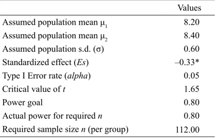
We enter the values in the Power Analysis module of the STATISTICA software and obtain results as in Table 1.
Table 1. Sample size calculation for comparing two group
means with a t-test for independent samples
Values
Assumed population mean μ1 8.20
Assumed population mean μ2 8.40
Assumed population s.d. (σ) 0.60
Standardized effect (Es) –0.33*
Type I Error rate (alpha) 0.05
Critical value of t 1.65
Power goal 0.80
Actual power for required n 0.80
Required sample size n (per group) 112.00 * the minus is a consequence of entering the lower value (μ1) first The analysis shows that in a situation when the population effect size is Es = 0.33, a number of 112 individuals would be needed in each group to detect a statistically significant difference between them (at the 0.05 level) with a probability of 0.8 (or 80%). Note that at the pre-study stage the estimation of expected effect size may be less accurate, and also some data may turn out to be unusable. To compensate, an investigator may wish to increase the size of each group by 10-15%.
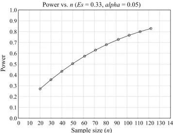
It may happen, however, that in many cases where the effects are small or medium researchers may report that no (statistically significant) differences were found. As a case in point, if we decided that the number of individuals in each group was 50 (i.e., 50 basketball players and 50 volleyball players), the probability of obtaining a significant result would not be much higher than 0.50 (50%). And, if there were only 30 individuals in each group, the chance of finding a significant difference would drop to 0.36 (36%). We illustrate the relationship between sample size and the power of this particular test in Figure 2 (for Es = 0.33, alpha = 0.05).
Power vs. n (Es = 0.33, alpha = 0.05) 0 10 20 30 40 50 60 70 80 90 100 110 120 130 140 Sample size (n) 0.0 0.1 0.2 0.3 0.4 0.5 0.6 0.7 0.8 0.9 1.0 P ow er
Figure 2. The power of a test as a function of sample size
(Es = 0.33, alpha = 0.05)
As already stated, the power of a test and the size of a sample in research depend on the population effect size. Now assume a different scenario. Suppose that the mean of volleyball players was μ2 = 8.7 sec (rather than μ2 = 8.4 sec). The difference between the group means has now become greater and equals Es = 0.83 (as expressed in standard deviation units). In such a situation, to detect an effect with an 80% chance
(power = 0.8), we would only need 19 individuals in
each group. Figure 3 illustrates the relationship between the effect size and sample size where there is an 80% chance of detecting an effect at the 0.05 alpha level
(power = 0.8, alpha = 0.05).
Of course, one-tailed tests may not always be appropriate. When in doubt, it is always preferable to adopt the more conservative non-directional hypothesis. As detailed earlier, if we planned to run a two-tailed test on our data (holding other criteria constant), the size of samples needed to detect an effect would increase. As shown in Table 2, to obtain an effect of Es = 0.33 with 0.8 probability, for a two-tailed t-test each group should contain 143 people.
Table 2. Sample size estimation for comparing two group
means with a two-tailed t-test for independent samples Value Assumed population mean (μ1) 8.20
Assumed population mean (μ2) 8.40 Assumed population s.d. (σ) 0.60
Standardized effect (Es) –0.33
Type I Error rate (alpha) 0.05
Critical value of t 1.97
Goal power 0.80
Actual power for required n 0.80 Required sample size n (per group) 143.00 Example 2. Comparing athletes from more than two sport disciplines
Here we will extend Example 1 a little further to compare athletes from more than two sport disciplines. Assume that now we aim to compare basketball players, volleyball players, and handball players in terms of their running time in a 60-metre sprint. Again, a thorough literature review and metanalysis are essential at this stage. This time we infer from previous reports that the means are likely to be as follows: μ1 = 8.0 sec (basketball players), μ2 = 8.2 sec (handball players), μ3 = 8.6 sec (volleyball players), and the population standard deviation is approximately σ = 0.6. We analyse the data with one-way analysis of variance (ANOVA). What sample size do we need to
detect an overall main effect of discipline?
A measure of the standardized effect size for ANOVA used in the STATISTICA software to calculate the power of a test and a required sample size is the RMSSE (Root Mean Square Standardized Effect). The RMSSE is an effect from the d family of size effects. For reasons of space and clarity, we will not go into detail about how this effect is computed. Suffice it to mention that we interpret its value as the standardized mean difference (measured in standard deviation units) between each group mean and the grand mean [28, 29, 30]. It is n vs. Es (power = 0.8, alpha = 0.05)
0.2 0.3 0.4 0.5 0.6 0.7 0.8 0.9 1.0
Standardized effect (Es) 0 20 40 60 80 100 120 140 160 R e qui re d s am pl e s iz e (n1 = n2 )
Figure 3. Sample size required to detect an effect with pow-er = 0.8 as a function of standardized effect size (alpha = 0.05,
two-tailed test) 1.0 0.9 0.8 0.7 0.6 0.5 0.4 0.3 0.2 0.1 0.0 Power
Power vs. n (Es = 0.33, alpha = 0.05)
0 10 20 30 40 50 60 70 80 90 100 110 120 130 140 n vs. Es (power = 0.8, alpha = 0.05) Sample size (n) 160 140 120 100 80 60 40 20 0
Required sample size (
n1
=
n2
)
Standardized effect (Es)
conventional to assume that an RMSSE of 0.15 is considered a small effect, a value of 0.3 is medium, and an RMSSE of 0.5 reflects a large effect. In our example, RMSSE is 0.51. However, researchers do not need to enter the RMSSE themselves as the software calculates the RMSSE once the assumed means and the population standard deviation have been entered.
Three sport disciplines (basketball, handball, and volleyball) were in this case entered as fixed factors (i.e., the three disciplines were selected purposefully, rather than chosen at random). Table 3 below shows (among other details) the estimated size of groups for the power of 0.8, alpha = 0.05, and gives the means and standard deviations in the population.
Table 3. Sample size estimation for comparing three group
means with one-way ANOVA
Value
Number of groups 3.00
Assumed RMSSE in population 0.51
Noncentrality parameter (delta) 5.19
Type I Error rate (alpha) 0.05
Power goal 0.80
Actual power for required n 0.81
Required sample size (n) (per group) 20.00 As detailed in Table 3, to detect an effect with a 0.8 chance (80%), we need 20 individuals in each group. Again, note that in order to ensure more confidence in detecting an effect, a researcher may want to increase the size of each group by 10-15%.
Example 3. Testing a two-way interaction effect Imagine that there is some scientific basis for assuming that motor abilities in junior and senior athletes differ relative to a sport discipline. For instance, the difference in the standing long jump of juniors and seniors is greater in discipline A than in discipline B. Such a complex effect is called a two-way interaction effect. Assume that in discipline A the expected means in the population are: μ1 = 180 cm for juniors, and μ2 = 210 for seniors. The corresponding means in discipline B are: μ3 = 180 cm (juniors), and μ4 = 190 cm (seniors). Assume further that the population standard deviation is 30 cm (σ = 30 cm). We ask How big do our samples need to be to detect
this interaction effect with an 80% probability (0.8)?
Now, in the STATISTICA software, where factors (sport
discipline: A, B; age category: junior, senior) are defined by rows and columns, we enter our data (our means and σ) into the columns and rows. The analysis produces information presented in Table 4.
Table 4. Sample size estimation involving a two-way
inter-action effect (two-way ANOVA)
Value
Number of rows 2.00
Number of columns 2.00
Type I Error rate (alpha) 0.05
Power goal 0.80
Interaction effect:
Assumed RMSSE in population 0.33
Actual power for required n 0.80
Required sample size (n) 72.00
As detailed in Table 4, to have an 80% chance (0.8) of detecting an effect, we would need 72 individuals in each of the four groups (Group 1: discipline A, juniors; Group 2: discipline A, seniors; Group 3: discipline B, juniors; Group 4: discipline B, seniors). Statistica’s Power Analysis module also computes required sample sizes for the two main factors, but we omit these here, as the logic is exactly the same as in the previous example. Example 4. Correlation between two variables Let us assume that we want to examine the relationship between a specific motor ability and sport performance in a particular test in football players (using a quantitative measure of effectiveness, say time). To determine the strength and direction of the relationship we examine, we use the Pearson’s correlation coefficient (r). Assume that our literature review has identified somewhat consistent findings showing that we can expect an
r = –0.45. Assume further that the theoretical grounds
for using a one-tailed test are solid and sufficient. Again, we ask How big a sample is enough?
Table 5. Sample size estimation for a correlation coefficient
using a one-tailed test
Value Assumed correlation in population (Ro) –0.45
Type I Error rate (alpha) 0.05
Goal power 0.80
Actual power for required n 0.82
As shown in Table 5, this time the sample size of 30 would be enough to detect an effect with an approximately 80% chance (0.8). If a two-tailed test was conducted, the sample would have to be bigger (as explained earlier),
n = 36 (see Table 6).
Table 6. Sample size estimation for a correlation coefficient
using a two-tailed test
Value Assumed correlation in population (Ro) –0.45
Type I Error rate (alpha) 0.05
Goal power 0.80
Actual power for required n 0.81
Required sample size (n) 36.00
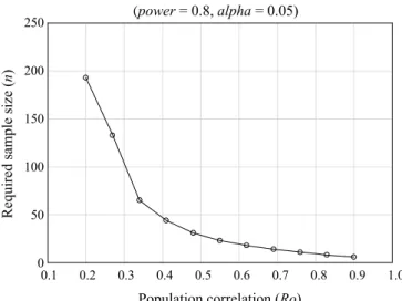
As mentioned earlier, the smaller the effect size, the greater the sample size that is needed to detect the effect (with all other factors kept constant, that is power = 0.8,
alpha = 0.05, two-tailed test) (see Figure 4).
(power = 0.8, alpha = 0.05)
0.1 0.2 0.3 0.4 0.5 0.6 0.7 0.8 0.9 1.0
Population correlation (Ro) 0 50 100 150 200 250 R equi red s am pl e s iz e ( n)
Figure 4. Required sample size to detect an effect with pow-er = 0.8 as a function of the size of the correlation coefficient
(alpha = 0.05, two-tailed test)
Example 5. Verifying the relationship between several independent variables and one dependent variable Let us assume that we study the relationship between several psychological traits and effectiveness. Psychological traits may embrace: emotional reactivity (negatively related to resistance to stress), achievement
motivation, and the level of aggression. The traits are
evaluated with the use of appropriate questionnaires, where a specific score on a scale is an indicator of a specific trait, and the score calculated from the official
qualification list is an indicator of effectiveness. In such a situation we often conduct a multiple regression analysis. Assume that previous research has revealed that these three predictors account for approximately 35% of the variance in effectiveness. How large does
our sample need to be, so that we would detect the effect with 0.8 probability?
Table 7. Sample size estimation for multiple regression
anal-ysis – a relationship between three independent variables and one dependent variable
Value
Number of predictors 3.00
R2 for null hypothesis (H
0) 0.00
Assumed R2 in population 0.35
Type I Error rate (alpha) 0.05
Goal power 0.80
Actual power for required n 0.80
Required sample size (n) 27.00
Table 7 shows that to detect an effect with an 80% chance (0.8), a sample size of 27 individuals is required. Required sample size is also dependent on the number of predictors, i.e. the bigger the number of predictors, the greater the sample size needed for the study. In our example, we estimate the power of a test only for the squared multiple correlations for the Omnibus
F-test. Thus, in our case, when using a sample size
as small as 27, it may happen that we will not detect a relationship between a particular predictor and the dependent variable (with other predictors held constant). Therefore, an estimated sample size should be larger. Some authors recommend that for regression analysis 10 individuals per one predictor is an absolute minimum (hence, 30 in our example with 3 predictors). Other authors claim, however, that even a sample size of 10 per predictor is not enough.
Step by step summary: How to use power analysis to estimate required sample size
As detailed earlier, a number of steps can be taken even before any data are collected to estimate an appropriate sample size needed for a study. To determine an adequate (optimal) sample size for your study [see 4, 17, 18]:
1. Analyse the theoretical premises and studies done hitherto that address your topic of interest. Estab-(power = 0.8, alpha = 0.05)
Population correlation (Ro)
0.1 0.2 0.3 0.4 0.5 0.6 0.7 0.8 0.9 1.0 250 200 150 100 50 0
Required sample size (
lish what is already known about the topic. As you continue to review the literature, try to identify the grounds behind a given difference, correlation, etc. (whether they are substantively and scientifically justified). Note down or compute estimates of effect size (e.g., differences between the means expressed in standard deviation units, a correlation coefficient, etc.). To compute effect size, you will often need mean values and a measure of variability (see [20] for details).
2. Formulate the null hypothesis and reflect on what form the alternative hypothesis will take. Drawing on theoretical premises, decide whether your alternative hypothesis will be directional or non-directional. For instance, judge whether the direction of a difference between the means or a correlation can be justified in a legitimate and substantive way.
3. Decide what statistical test to use to verify the sta-tistical hypotheses.
4. Specify the level of significance (alpha). A common practice in sport, medical, and social sciences is to
set alpha at 0.05.
5. Decide on the desired test power. In sport sciences the power is often specified at 0.8.
6. Determine the required sample size. What this paper adds?
The paper emphasises the need to consider the power of a test in sport sciences. The authors discuss the main assumptions behind statistical power analysis, and demonstrate through hypothetical examples from sport sciences how to estimate the required sample size at the pre-study stage. The examples illustrate statistical hypothesis verification with the use of independent-sample t-test, one-way and two-way analysis of variance, correlation analysis, and multiple regression analysis.
References
1. Kleka P. Statystyczne kryteria przydatności raportu do metaanalizy (Usefulness of statistical parameters for metaanalysis). In: Brzeziński J, ed., Metodologia badań społecznych. Wybór tekstów (Methodology of social research. A selection of texts). Poznań: Zysk i S-ka. 2011: 99-114.
2. Fritz CO, Morris PE, Richler JJ. Effect size estimates: current use, calculations, and interpretation. J Exp Psychol Gen. 2012; 141(1): 2-18.
3. Ferguson GA, Takane Y. Analiza statystyczna w psychologii i pedagogice (Statistical analysis in psychology and education). Warszawa: Wydawnictwo Naukowe PWN. 2007.
4. King BM, Minium EM. Statistical reasoning in psychology and education. 4th ed. Hoboken, NJ: John Wiley & Sons, Inc. 2003.
5. Cohen J. A power primer. Psychol Bull. 1992; 112(1): 155-159.
6. Cohen J. Statistical power analysis for the behavioral sciences. 2nd ed. Hillsdale, NJ: Lawrence Erlbaum. 1988. 7. Seltman HJ. Experimental design and analysis.
Pittsburgh: Carnegie Mellon University. 2012.
8. Kaplan D. The SAGE handbook of quantitative methodology for the social sciences. London, UK: Sage Publications, Inc. 2004.
9. Good PI. Resampling methods: a practical guide to data analysis. 3rd ed. Boston, MA: Birkhäuser. 2005. 10. Kraemer HC, Thiemann S. How many subjects?: Statistical
power analysis in research: Sage Publications, Inc. 1987. 11. Ajeneye F. Power and sample size estimation in research.
Biomed Sci. 2006; 50: 988-990.
12. Hill R. What sample size is “enough” in internet survey research? IPCT-J. 1998; 6(3-4): 1-12.
13. Houser J. How many are enough? Statistical power analysis and sample size estimation in clinical research. J Clin Res Best Pract. 2007; 3(3): 1-5.
14. Martínez-Mesa J, González-Chica DA, Bastos JL, et al. Sample size: how many participants do I need in my research? An Bras Dermatol. 2014; 89(4): 609-615. 15. Eng J. Sample size estimation: How many individuals
should be studied? Radiology. 2003; 227(2): 309-313. 16. Burmeister E, Aitken LM. Sample size: How many is
enough? Aust Crit Care. 2012; 25(4): 271-274.
17. Wątroba J. Przystępnie o statystycznym podejściu do testowania hipotez badawczych i szacowania liczebności próby. StatSoft Polska. 2011: 33-43.
18. Wątroba J. Praktyczne aspekty szacowania liczebności próby w badaniach empirycznych. StatSoft Polska. 2013: 5-15.
19. Brzeziński J. Metodologia badań psychologicznych (Methodology of psychological research). Warszawa: Wydawnictwo Naukowe PWN. 1996.
20. Tomczak M, Tomczak E. The need to report effect size estimates revisited. An overview of some recommended measures of effect size. TSS. 2014; 21(1): 19-25. 21. Aranowska E, Rytel J. Istotność statystyczna – co to
naprawdę znaczy? (Statistical significance – what does it really mean?). 1997; 40(3-4): 249-260.
22. Levine G, Parkinson S. Experimental methods in psychology. New York, NY: Psychology Press. 2014. 23. Aberson CL. Applied power analysis for the behavioral
sciences. New York, NY: Routledge. 2010.
24. Olinsky A, Schumacher P, Quinn J. The importance of teaching power in statistical hypothesis testing. Int J Math Teach Learn. 2012; 1.
25. Wilson VanVoorhis CR, Morgan BL. Understanding power and rules of thumb for determining sample sizes. Tutor Quant Methods Psychol. 2007; 3(2): 43-50. 26. Borkowf CB, Johnson LL, Albert PS. Power and sample
size calculations. In: Gallin JI and Ognibene FP, eds., Principles and practice of clinical research. Amsterdam: Academic Press. 2012: 271-283.
27. Rosner B. Fundamentals of biostatistics. 7th ed. Boston, MA: Brooks/Cole Cengage Learning. 2011.
28. Howell DH. Statistical methods for psychology. Belmont, CA: Wadsworth, Cengage Learning. 2012.
29. Steiger JH. Beyond the F test: Effect size confidence intervals and tests of close fit in the analysis of variance and contrast analysis. Psychol Methods. 2004; 9(2): 164-182.
30. Steiger JH, Fouladi RT. Noncentrality interval estimation and the evaluation of statistical models. In: Harlow LL, Mulaik SA, and Steiger JH, eds., What if there were no significance tests? Mahwah, NJ: Erlbaum. 1997: 221-257.