Models for solving the tariff optimization problem

MODELS FOR SOLVING THE TARIFF OPTIMIZATION

PROBLEM

Radosław Pytlak* and Wojciech Stecz**

*

Institute of Automatic Control and Robotics, Warsaw University of Technology, Sw. Andrzeja Boboli 8, 02-525 Warsaw, Poland, r.pytlak@mchtr.pw.edu.pl ** Faculty of Cybernetics, Military University of Technology, Kaliskiego 2, Warsaw,

Poland, wojciech.stecz@wat.edu.pl

Abstract We present the methods of telecommunication tariff optimization from a point of client’s view. A client which wants to minimize his monthly fees tries to choose a proper tariff model. In case of large companies these models are more complicated and the optimization models should be used. We describe a simple MIP models and their modifications solved with CLP solvers. All the examples were solved with ILOG and ECLiPSe MIP and CLP solvers.

Paper type: Research Paper Published online: 30 April 2014 Vol. 4, No. 2, pp. 119-133 ISSN 2083-4942 (Print) ISSN 2083-4950 (Online)

© 2014 Poznan University of Technology. All rights reserved.

1. TARIFF OPTIMIZATION IN TELECOMMUNICATION

1.1 Introduction

The problem we consider is related to the selection of an optimal tariff offered to a customer by a telecommunication company. A customer aims at choosing the best (usually the low cost) tariff from available offers. Because of structure of the tariffs the customer can have problems in a proper estimation of the future tariff costs and as a result he can miss the optimal tariff. A telecommunication company proposes the combinations of services within several contracts to an indi-vidual customer or a corporation. Among these services are for example: domestic and foreign calls, local and long distance calls, SMS and MMS messages, etc. In general the number of these services can be quite significant especially when a corporate client is considered. Some of these services can be packed into packages which we call contracts -- they require fixed monthly payments if the specified number of services included in them are not exceeded. If a customer uses more services than those specified in the contract he is charged for each exceeding service. The tariff optimization problem is then defined as a problem of finding the best possible choice of contracts such that the monthly client payment is the lowest.

The tariff optimization problem can also be considered from the telecom-munication operators point of view. In that case one tries to maximize revenue in the telecommunication network he manages. These optimization models propose how to deal with the yield management. Yield management has attracted interest from theoretical as well as operational point of view0. One may assume that this can be seen as elaborating the pricing strategies using maximum capacity available to the telecommunication operator. Bouhtou et al. studied pricing for telecommuni-cations and proposed a model of multilevel pricing0. Another approach was0 a bi-level optimization formulation to model competition between operators. Viterbo et al.0 described revenue maximization during a real-time pricing for cellular network operator. Bouhtou 0 considered a pricing model for the operator that owns a subset of telecommunication routes and receives a revenue by allowing clients to use them. Multiply clients which use telecommunication network choose the routes taking into account the costs of the communication routes.

None of above described models can be used by companies which use telecommunication services and sign a contract with a telecommunication company which should provide the lowest possible costs of these services.

We assume that a customer knows his own profile. By the customer's profile we mean his average use of services during some pre-specified period of time (usually last year data are considered). Taking into account only some telecom-munication offers in the national market we can stress that these offers very often involve a mechanism of discounts for clients and that mechanism can be only modeled by using logic programming techniques.

In this article we describe some optimization problems which are derived from a base problem by adding constraints (not only logical constraints but also con-straints that can be described as logical predicates with first order predicate logic). All the presented problems were modeled and solved in CISCO ECLiPSe and IBM ILOG CPLEX environments. The first environment uses a classic CLP solver while the second one applies MIP/QP solver with constraint programming techniques involved.

1.2 Problem formulation

In this section we present a formal definition of the tariff optimization problem. First a MILP (Mixed Integer Linear Problem) model is presented. This model is the basis for the optimization problems solved by ILOG and ECLiPSe solvers. Next the model is modified by the introduction of some logic constraints and general logic programming constraints like alldifferent. A base problem is thus transformed into a constraint logic programming problem that can be solved by CLP solvers or hybrid MILP – CLP solvers as the next sections show.

Let us denote by

y

i the number of contracts of the i-th type and by xij the number

of the j-th services within the i-th type of contract. Then the tariff optimization problem – P - is as follows (more general formulations with the option for substitute services are possible)





 

 



















m i n j ij i ij ij i i i i y x

c

y

c

v

c

x

y

b

1 1 0 ,

max

0

,

min

(1) subject to:



   m i h j ij x j n x 1 ,..., 1 , (2)









n j i ij

M

y

i

m

x

1 1

,...,

1

,

(3)

m

i

L

y

_i



_i

,



1

,...,

(4) m i v M y_i 2_i, 1,..., (5) n j m i xij, 1,...,, 1,..., 0   (6)

Here, x



xiji1,...,m,j1,...,n, y

 

yi i1,...,m,

c

i is the monthly cost of the i-th

contract, cij is the unit cost of the j-th service in the i-th contract and bij is the limit of

the j-th service in the i-th contract which is included in the contract as free of charge. Furthermore, xhj denotes the average number of units of the j-th service measured

in the pre-specified period of time. ci0 is a monthly cost of using contracts from

a company point of view. It may be treated as additional costs put on the contract signed. Then

v

i describes situation that additional costs are paid when contract is

signed (

v

i is a Boolean variable).

In order to complete the description of the problem we have to indicate that variables

y

are integer variables, furthermore we assume that x are real numbers. Problem P can be stated as a standard linear MILP problem by introducing auxiliary variables zij which transform the problem to the problem with a

differen-tiable cost function (IBM ILOG,2009):























m i ij ij i i i i y x

c

y

c

v

c

z

1 0 ,

min

(7) subject to:

n

j

m

i

z

b

y

x

_ij



_iij



_ij



0

,



1

,...,

,



1

,...,

(8)

n

j

m

i

z

ij

,

1

,...,

,

1

,...,

0







(9) and constraints (2)-(6).

2. SOLVING A TARIFF OPTIMIZATION PROBLEM

2.1. MIP models

In this section we present a base formulation of the tariff optimization problem and some of its modifications. We introduce additional logic constraints Bouhtou, Medori & Minoux, 2011) and global predicates alldifferent (CISCO Systems, 2006). Logic constraints were not transformed into algebraic equations, because in a general case it may by a time consuming task (Fruwirth & Abdennadher, 2003).

A tariff optimization problem (1)-(6) is a standard MIP problem (in this case MILP problem), where all the constraints are linear and an optimization function is a linear function too. This model can be easily solved and one have a guarantee that a solution found will be an optimal solution (or that there is no bounded solution). Linear MIP problems can be solved very effectively by modern solvers such as IBM ILOG or ECLiPSe solver. When we have to reformulate the problem by adding logical constraints we can try to remodel the problem by putting the logical constraints as algebraic constraints.

Some modern solvers like ILOG have their own mechanisms that automatically reformulate the logic constraints to the algebraic ones (CISCO Systems, 2006) (Fruwirth & Abdennadher, 2003). If it is not the case one must do it manually and that can be difficult. Fortunately ILOG CPLEX allows us to formulate MIP problems with logic constraints and solve it with a modified MIP solver.

2.2. Decomposition method for MIP problem

Problem P can be solved by various algorithms (some results are presented in the next section), however for problems with large m and n the performance of these methods couldn't allow us to use them in on-line computations – when this task is solved by the telecommunication companies (an offer for a corporate client can refer to as many as 20 different contracts which can have as many as 200 different services).

In order to circumvent the dimensionality problem we advocate to use the rela-xation methods based on the Lagrangian of the problem. Since only constraints (2) unable us to solve the problem in the decomposed way-each subproblem corresponds to each contract i-th-we introduce the Lagrange function with respect to these constraints:

 

_

_

_

_

   













_





















n j m i h j ij j m i n j ij ij i i i i

y

c

v

c

z

x

x

c

y

x

f

1 1 1 1 0

,

,

~





(10)

where



jare the Lagrange multipliers corresponding to (2).

The problem can then be solved by using two-stage algorithm where at the lower level subproblems

P

i

,

i



1

,...,

m

are solved:

 







































  h j ij j n j ij ij i i i i z x y_{iijijj n}

c

y

c

v

c

z



x

x

1 0 ,

min

_,,1,..., (11)

subject to (2)-(6) and (8)-(9) and assuming that



j,j1,...,n from the upper level

At the upper level of the algorithm variables



j,j1,...,n are updated in order to

maximize the function f





~f



x

 



,y



,





.

Where x

 



and y

 



are solutions to the problems

P

i

,

i



1

,...,

m

. Since the

upper level of the optimization algorithm is nondifferentiable problem subgradient methods such as those described in (Goncalves & Ladanyi, 2005) should be used to solve it. The subgradient method we propose to solve the upper optimization problem is that of Kiwiel (Kiwiel, 1985).

2.3. ILOG CPLEX problem formulation

Below we present the problem formulation in which only algebraic constraints were taken into account. The problem is described in OPL – modern language for modeling the optimization problems formulated within ILOG. First the parameters and variables definitions are presented.

int NbContracts = ...; int NbServices = ...;

range Contracts = 1..NbContracts; range Services = 1..NbServices;

float ContractCosts[Contracts] = ...; float ContractServicesCosts[Contracts,Services] = ...; float ContractInitialCosts[Contracts] = ...; float Xh[Services] = ...; float M[Contracts] = ...; float b[Contracts,Services] = ...; dvar int+ y[Contracts];

dvar int+ z[Contracts,Services]; dvar int+ x[Contracts,Services]; dvar int+ v[Contracts] in 0..1;

Variable dvar int+ means that a variable is a positive integer. Optimization function (7) can be modeled as:

minimize

sum(i in Contracts) ContractCosts[i]*y[i] + sum(i in Contracts, j in Services) ContractServicesCosts[i,j]*z[i,j] +

sum(i in Contracts ) ContractInitialCosts[i]*v[i];

Constraints (2)-(6) and (8)-(9) can be modeled as: subject to {

forall( j in Services ) c_hist_data:

forall( i in Contracts ) c_yx_connection:

sum(j in Services) x[i][j] <= M1*y[i]; forall( i in Contracts )

c_contracts_limit: y[i] <= M[i]; forall( i in Contracts )

sum( j in Services ) z[i][j] >= 0.0; forall( i in Contracts, k in Services ) x[i][k] - y[i]*b[i][k] - z[i][k] <= 0.0; forall( i in Contracts )

c_v_data: y[i] <= M2*v[i]; }

OPL language can be used to model both MIP and CLP problems. We have to stress that there are interfaces between OPL and other languages (.NET, JAVA or C++).

2.4. CLP problem formulation

CLP (Constraint Logic Programming) is an alternative method we can use to solve the tariff optimization problem. A CLP method is, for example, discussed in and is used to solve the combinatorial problems where some of the constraints cannot be formulated as algebraic equations. These constraints are very often modeled as standard global predicates like alldifferent, atleast, atmost etc.

CLP calculus is a generalization of LP (Logic Programming). The only modification in CLP are the added constraints, so the unification is replaced by constraint handling process. Constraints can occur in the goals rule and in the body clauses. Clauses of CLP and LP (Logic Programming) are defined in the same way. CLP syntax is presented in (11).

The optimization problem P can also be stated as a CLP model in ECLiPSe. The variables and parameters definitions are the same as in ILOG solver. Constraints and optimization function are shown below. ECLiPSe language is a Prolog language extension which allows sophisticated construction of constraints. Because CLP solver search for a solution and grounds the variables we must use

eval() predicate in order to evaluate terms in arithmetic expressions). This is one

of the predicates used by the ECLiPSe compiler to expand arithmetic expressions. The searching process is described in (Bouhtou,Erbs,Minoux,2007), (Bouhtou, Medori & Minoux, 2011). The modeling issues are described in (Nemhauser & Wolsey, 1988), (Pytlak & Stecz, 2007).

dim(Y,[NumContracts]), Y :: 0..Nc, dim(V,[NumContracts]), V :: 0..1, dim(X,[NumContracts,NumServices]), X :: 0..Ns, dim(Z,[NumContracts,NumServices]),

Z :: 0..Ns, /* constraints */ % constraint no. (for(I,1,NumContracts), param(NumServices,X,Y,Z,B) do (for(J,1,NumServices), param(X,Z,Y,B,I) do eval(X[I,J])-eval(Y[I])*B[I,J]-eval(Z[I,J]) #=< 0 )), % constraint no.

(for(I,1,NumContracts),param(Y,M) do eval(Y[I])#=< M[I]), % constraint no. (for(J,1,NumServices),param(NumContracts,Xh,X) do Xj is X[1..NumContracts,J], eval(sum(Xj)) #= Xh[J]), % constraint no. (for(I,1,NumContracts), param(NumServices,Y,X,M1) do Xi is X[I,1..NumServices], eval(sum(Xi)) #=< M1*Y[I]), % coinstraint no. (for(I,1,NumContracts), param(NumServices,Z) do Zi is Z[I,1..NumServices], eval(sum(Zi)) #>= 0), % coinstraint no. (for(I,1,NumContracts), param(Y,V,M2) do eval(Y[I]) #=< M2*eval(V[I])), /* optimization criteria */

% elements of min function – Costs1, Costs2, Costs3 (for(I,1,NumContracts), fromto(0,In1,In1+ContractCosts[I] * Y[I],Costs1), param(Y,ContractCosts) do true), (for(I,1,NumContracts) * for(J,1,NumServices), fromto(0,In,Out,Costs2), param(ServiceCosts,Z) do

Out = In + ServiceCosts[I,J] * Z[I,J]), (for(I,1,NumContracts), fromto(0,In1,In1+ContractInitialCosts[I] * V[I],Costs3), param(V,ContractInitialCosts) do true), TotalCosts #= eval(Costs1)+eval(Costs2)+eval(Costs3), term_variables([V,Y,X,Z,TotalCosts], Vars), /* search algorithm */ bb_min(search(Vars,0,first_fail,indomain_min,bbs(100), [backtrack(Backtracks)]),TotalCosts, bb_options{strategy:dichotomic, timeout:260})

Function bb_min starts a branch and bound solver on interval constraints (IC ECLiPSe library). Its aim is to make it convenient to write hybrid solutions to

problems, mixing together integer and real constraints and variables. Search method (method of instantiation of variables) search is configured to search the variables with the smallest domains. Algorithm start searching from the middle of the variable domain.

2.5. Additional constraints: logic constraints and global predicates

Very often one is not able to model optimization problems as MIP or MILP problems, because additional constraints should be taken into account that are not algebraic ones. For example, consider logic constraints and one global predicate

alldifferent that should be included in the discussed model. The logic constraints

are of the form (16) and (17) as presented below.











_k j

y

y

(12)











_k h j

y

x

(13)

Both (15) and (16) constraints prevent solver from setting any value to

y

k from its

domain. Both ILOG CLPEX and ECLiPSe solvers were able to find solutions when these constraints were added. ILOG CLPEX transformed these constraints to the algebraic ones automatically so we could solve this problem with standard MIP and CP solver. Parameters



,



were set by taking into account historical usage of services.

The global constraint alldifferent enforces all variables to take distinct values. The alldifferent constraint occurs in most practical problems directly or indirectly. A first example is the n-queen chess puzzle problem when one has to place n que-ens on a n by n chessboard in such a way that no queen attacks another. Two queens attack each other if they are located on the same column, on the same row, or on the same diagonal. One way of solving this problem is to model it as

theconjunction of three alldifferent constraints.

2.6. Hybrid problem formulation (MIP and CLP)

Hybrid solvers that link MIP (or MILP) and CLP solver functionality must communicate in effective way to obtain feasible solutions and later to find the optimal/suboptimal solution. To fulfill this assumption one has to combine the availability of the MIP solver with an event-driven execution by the CLP solver in order to achieve a mutual cooperation for solving linear and other constraints. Hybrid solver has to be able to detect inconsistency of a problem and to propagate information in case of consistency.

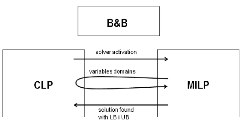
The MIP solver is automatically invoked by Branch & Bound steering mechanism when the corresponding constraint system has been changed (by CLP

solver). There are precisely defined situations when MIP solver is invoked. These are: when CLP solver adds a new linear constraint, CLP solver finds tighter / better variable bounds (then the previously found solution is excluded) or when any variable is instantiated of variables to a value different from its solution value (search and ground process is described in (Nemhauser & Wolsey, 1988)). The in-formation flow between CLP and MIP solvers is shown in Fig. 1.

Fig. 1 Framework of hybrid MIP and CLP solver

The main steps during hybrid solver computations are: 1. Constraints settings (for the variables and domains) 2. Search methods settings (problem specific)

3. Constraint propagation (depends on domain: IC, FD) domain bounding, searching for empty domains, variables grounding

4. Solving relaxed MIP problem checking a solution at each node, checking optimum values according to lower and upper bounds.

Steps 3-4 are made until the solution is found.

The optimization problem P, as a hybrid CLP-MIP model in ECLiPSe, is presented below. The communication model between MIP and CP solvers (a hybrid solver model) is described in 2.7.

dim(Y,[NumContracts]),

[eplex, ic]: (Y[NumContracts] $:: 0.0..T), [eplex, ic]: (integers(Y[1..NumContracts])), dim(V,[NumContracts]), [eplex]: (V[NumContracts] $:: 0.0..1.0), [eplex]: (integers(V[1..NumContracts])), dim(X,[NumContracts,NumServices]), [eplex]: (X[NumContracts,NumServices] $:: 0.0..M), dim(Z,[NumContracts,NumServices]), [eplex]: (Z[NumContracts,NumServices] $:: 0.0..N),

Eplex MILP solver can be changed and many commercial and open source solvers can be added (CPLEX, COIN-OR project solvers etc.). In our case it was

COIN-OR CBC MIP solver. ECLiPSe can be assigned to ILOG solver as MIP solver too. One has to assign very carefully each constraint to the constraint solver. A constraint can be assigned to more than one solver.

/* MIP constraints */

(for(I,1,NumContracts), param(NumServices,X,Y,Z,B) do (for(J,1,NumServices), param(X,Z,Y,B,I) do

eplex: (X[I,J] - Y[I]*B[I,J] - Z[I,J] $=< 0.0))), (for(I,1,NumContracts), param(NumServices,X,Z) do (for(J,1,NumServices), param(X,Z,I) do

eplex: (X[I,J] $>= 0.0), eplex: (Z[I,J] $>= 0.0))),

(for(I,1,NumContracts), param(Y,V) do [eplex, ic]: (Y[I] $>= 0.0),

[eplex, ic]: (Y[I] $=< 100.0), eplex: (V[I] $>= 0.0),

eplex: (V[I] $=< 1.0)),

(for(J,1,NumServices), param(NumContracts,Xh,X) do eplex: (sum(X[1..NumContracts,J]) $= Xh[J])), (for(I,1,NumContracts), param(NumServices,Y,X,M1) do eplex: (sum(X[I,1..NumServices]) $=< M1*Y[I])),

(for(I,1,NumContracts), param(Y,V,M2) do eplex: (Y[I] $=< M2*V[I])),

/* CLP constraints */ ic: (Y[9] $=< 10),

ic: (alldifferent(Y[1..3])), ic: (Cost $>= 0.0),

/* optimization criteria */

!!! The same as in MIP solver case

eplex: (TotalCosts $= Costs1 + Costs2 + Costs3), /* search algorithm */

eplex_solver_setup(

min(TotalCosts),Cost,[sync_bounds(yes)],inst]),

bb_min((labeling(Y),eplex_get(cost,Cost)),Cost,bb_options{strategy :continue}).

Branch and bound search algorithm starts the MIP solver and solves the MIP task. Next the labeling process is started and CLP solver propagates the constraints. When Y vector values change, B&B algorithm restarts MIP solver with the new Y vector with the smaller domains for its elements. The process is conducted till all CLP constraints are satisfied and MIP solver finds a solution (or finds an inconsistency).

3. NUMERICAL RESULTS

We applied our optimization model in small and medium size problems. Below we present the results for medium optimization tests.

Table 1 Results for MIP ILOG CPLEX solver

Optimization of medium problems Number of variables: 1327 (13 contracts and 50 services) MILP problem CPU time [s] number of

iterations

number of cuts without logic constraints 0.47 1056 188 with logic constraints 0.20 373 11

Relatively good results for the second problem with the logic constraints can be explained by the fact that the addition of the logic constraints narrows the search space. These results suggest that introducing these constraints can speed up the search process. However, this is not the rule in a general case.

In the Table 2 the results of the CLP solver are presented. All the variables were defined as integers which improved a search process performance. In the other case, when variables were the Real numbers, CLP solver needed more CPU time.

Table 2 Results for CLP ILOG CPLEX solver

Optimization of medium optimization task Number of variables: 1327 (13 contracts and 50 services) CLP problem CPU time [s] number of

branches

number of failures without logic constraints 120.0 216.000 >97.000 with logic constraints 120.0 214.000 >97.000 with logic constraint and

alldifferent (Y[1..3])

predicate

(time not acceptable) 179.000 >70.000

The experiments show that the proper setup of optimization solvers is crucial for solving problems efficiently (see (Pytlak & Stecz, 2007) for details). In our experiments the presented results show that using CP solver to MIP problems can’t guarantee good and acceptable solution. We need 2 stage hybrid algorithm which first solves the MIP problem and then try to correct this solution by taking into accunt global LP predicate as alldifferent.

Table 3 Results for CLP ECLiPSe solver

Optimization of medium problems Number of variables: 1620 (10 contracts and 80 services)

CLP problem CPU time [s] Search strategy:

most_constrained

Search strategy:

Occurrence

without logic constraints 23.0 18.85 with logic constraints 20.85 (time not acceptable) with logic constraints

and alldifferent (Y[1..3)]) predicate

(time not acceptable) (time not acceptable)

If one puts no limits on the number of contracts that can be chosen then CP solver searches the tree efficiently. But when we put the limits on the number of contracts the solver cannot find a solution in less than 10 minutes. This time is not acceptable.

Search process (domain search strategy) was set to most_constrained. The entries with the smallest domain size were selected. This strategy assumes that if several entries have the same domain size, the entry with the largest number of attached constraints is selected. Occurrence search strategy selects the entry with the largest number of attached constraints. Another good strategy is dbs search strategy. The depth bounded search explores the first k choices in the search tree completely. After that it switches to another search method.

Table 4 Results for hybrid ECLiPSe solver

Optimization of medium problems Number of variables: 1620 (10 contracts and 80 services)

CLP problem CPU time [s]

B&B search strategy:

continue

B&B search strategy:

Dichotomic

with logic constraints 13.0 25.0 with logic constraints

and alldifferent (Y[1..3]) predicate

39.9 82.0

Presence of the predicate alldifferent causes that the solver hardly finds the solution. Some additional logic constraints may help to constrain the search space however the global predicates are the most difficult procedures solved by the CLP or hybrid solvers. Therefore if the global predicates are not needed they should be omitted.

4. CONCLUSION

The paper presents a practical problem of determining an optimal tariff for a customer of a mobile telecommunications company. The problem is formulated from a customer point of view. Because telecommunication company offers can be

complicated the potential client must be able to model these propositions in order to choose the tariff with an optimal cost.

By taking into account the need for modeling complicated problems we used the constraint logic programming as a tool for handling constraints such as logical constraints. Some modern optimizations solvers were discussed in the paper and several optimization problems were solved.

REFERENCES

Bouhtou M., Erbs G. & Minoux M., (2007), Joint optimization of pricing and resource allocation in competitive telecommunications networks. Networks 50 pp. 37- 49. Bouhtou M., Medori J., Minoux M., (2011), Mixed Integer Programming model for pricing

in telecommunication, INOC 2011, Hambourg : France.

Bouhtou M., Hoesel S., Kraaaij A. & Lutton J., (2003), Tariff optimization in networks, INFORMS Journal on Computing; Vol. 19 Issue 3, p. 458.

CISCO Systems, (2006), ECLiPSe User Manual ver.6.0.

CISCO Systems, (2006), ECLiPSe Tutorial Introduction ver.6.0 (2006).

Fruwirth T. & Abdennadher S., (2003), Essentials of constraint programming, Springer. Goncalves, J.P.M. & Ladanyi, L., (2005), An Implementation of a Separation for Mixed

Integer Rounding Inequalities, IBM Research Report RC23686 August 2. IBM ILOG, (2009), ILOG OPL Language User’s manual ver.6.3.

IBM ILOG, (2009), User’s manual for CPLEX ver.12.2.

Kiwiel, K.C., (1985), Methods of descent for nondifferentiable optimization. Lecture Notes in Mathematics, Heidelberg, Springer—Verlag.

Nemhauser, G. & Wolsey, L., (1988), Integer and Combinatorial Optimization, Wiley Interscience.

Pytlak R. & Stecz W., (2007), Tariff optimization problem, IFIP 2007, EAIiE-AGH Cracow.

Simonis H., (2005), Developing Aplications with ECLiPSe, IC-Parc Technical Report-03-2 Wallace M., (2005), Hybrid algorithms, local search and ECLiPSe, CP Summer School. Wallace M. & Schimpf J., (2002), Finding the right hybrid algorithm – A combinatorial

meta-problem, Annals of Mathematics and Artificial Intelligence 34: pp. 259–269. Viterbo E. & Chiasserini C., (2001), Dynamic Pricing in Wireless Networks, 12th

International Symposium on Personal, Indoor and Mobile Radio Communications, San Diego, California, USA.

BIOGRAPHICAL NOTES

Radosław Pytlak is a Professor at Institute of Automatic Control and Robotics of

Warsaw University of Technology. He teaches: modeling, simulation and optimization of dynamical systems; numerical methods; theory and methods of nonlinear programming; scheduling. His interests lie mainly in dynamic optimization and in algorithms for large scale optimization problems. He is the author of two monographs published in Springer-Verlag: Numerical methods for

optimal control problems with state constraints; Conjugate gradient algorithms in nonconvex optimization. He published several papers in leading journals on optimization such as: SIAM J. on Optimization; SIAM J. on Control and Optimization; Journal of Optimization Theory and Applications; Numerische Mathematik.

Wojciech Stecz is an assistant professor at Faculty of Cybernetics Military

University of Technology. He teaches: modeling and simulation of systems; numerical methods; theory and methods of nonlinear programming and scheduling.