PMC-optimal nonparametric quantile estimator Ryszard Zieli´nski
Institute of Mathematics Polish Academy of Sciences
According to Pitman’s Measure of Closeness, if T1 and T2 are
two estimators of a real parameter θ, then T1 is better than T2 if
Pθ{|T1− θ| < |T2− θ|} > 1/2 for all θ. It may however happen that
while T1 is better than T2 and T2 is better than T3, T3 is better than
T1. Given q ∈ (0, 1) and a sample X1, X2, . . . , Xn from an unknown
F ∈ F, an estimator T∗ = T∗(X1, X2, . . . , Xn) of the q-th
quan-tile of the distribution F is constructed such that PF{|F (T∗) − q| ≤
|F (T ) − q|} ≥ 1/2 for all F ∈ F and for all T ∈ T , where F is a nonparametric family of distributions and T is a class of estimators. It is shown that T∗ = X
j:n for a suitably chosen jth order statistic.
AMS 1991 subject classification: Primary 62G05; secondary 62G30
Key words and phrases: quantile estimators, nonparametric model, optimal esti-mation, equivariant estimators, PMC (Pitman’s Measure of Closeness)
Address: Institute of Mathematics PAN, P.O.Box 137, 00-950 Warsaw, Poland E-mail: rziel@impan.gov.pl
Pitman’s Measure of Closeness If T and S are two estimators of a real parameter θ we define T as better than S if Pθ{|T − θ| ≤ |S − θ|} ≥ 1/2 for all θ
(Keating et al. 1991, 1993). A rationale behind that criterion is that the absolute error of estimator T is more often smaller than that of S. A restricted applicability of the idea is a consequence of the fact that while T1 is better than T2 and T2 is
better than T3 it may happen that T3 is better than T1. It may however happen
that in a given statistical model and in a given class of estimators there exists one which is better than any other. We define such estimator as PMC-optimal . In what follows we construct a PMC-optimal estimator of a qth quantile of an unknown continuous and strictly increasing distribution function.
Statistical model. Let F be the family of all continuous and strictly increas-ing distribution functions on the real line: F ∈ F if and only if F (a)=0,F (b)=1, and F is strictly increasing on (a, b) for some a and b, −∞ ≤ a < b ≤ +∞. Let X1, X2, . . . , Xn be a sample from an unknown F ∈ F and let X1:n, X2:n, . . .
. . . , Xn:n (X1:n ≤ X2:n ≤ . . . ≤ Xn:n) be the order statistic from the sample. The
sample size n is assumed to be fixed (nonasymptotic approach). Let q ∈ (0, 1) be a given number and let xq(F ) denote the qth quantile (the quantile of order q) of
the distribution F ∈ F. The problem is to estimate xq(F ).
Due to the fact that (X1:n, X2:n, . . . , Xn:n) is a minimal sufficient and
com-plete statistic for F (Lehmann 1983) we confine ourselves to estimators T = T (X1:n, X2:n, . . . , Xn:n).
Observe that if X is a random variable with a distribution F ∈ F with the qth quantile equal to x then, for every strictly increasing fucntion ϕ, the random variable ϕ(X) has a distribution from F with the qth quantile equal to ϕ(x). According to that property we confine ourselves to the class T of equivariant estimators: T ∈ T iff
T (ϕ(x1), ϕ(x2), . . . , ϕ(xn)) = ϕ (T (x1, x2, . . . , xn))
for all strictly increasing functions ϕ and for all x1 ≤ x2 ≤ . . . ≤ xn
It follows that T (x1, x2, ..., xn) = xk for any fixed k (Uhlmann (1963)).
estimators (1) is identical with the class of estimators T = XJ(λ):n
where J(λ) is a random variable independent of the sample X1, X2, . . . , Xn, such
that P {J(λ) = j} = λj, λj ≥ 0, j = 1, 2, . . . , n, n X j=1 λj = 1
This gives us an explicit and easily tractable characterization of the class T of estimators under consideration.
Observe that if T is to be a good estimator of the qth quantile xq(F ) of an
unknown distribution F ∈ F, then F (T ) should be close to q. Hence we shall measure the error of estimation in terms of differences |F (T (X1, X2, . . . , Xn))− q|
rather than in terms of differences |T (X1, X2, . . . , Xn)) − xq(F )|. According to the
Pitman’s Measure of Closeness an estimator T is better than S if (1) PF{|F (T ) − q| ≤ |F (S) − q|} ≥ 1/2 for all F ∈ F
(for more fine definitions see Keating et al. 1993). Definition. An estimator T∗ which satisfies
(2) PF{|F (T∗) − q| ≤ |F (S) − q|} ≥ 1/2 for all F ∈ F and for all S ∈ T
is said to be PMC-optimal .
We use ≤ in the first inequality in the above definition because for T = S we prefer to have LHS of (1) to be equal to one rather than to zero; otherwise the part ”for all T ∈ T ” in (2) would not be true. For example two different estimators X[nq]:n and X[(n+1)q]:n are identical for n = 7 when estimating qth quantile for q = 0.2.
One can easily conclude from the proof of the Theorem below that the second inequality ≥1/2 may be strengthened in the following sense: if there are two optimal estimators T∗
1 and T2∗ (we can see from the proof of the Theorem that it may
hap-pen), then PF{|F (T1∗)−q|≤|F (T2∗)−q|}= 1 2 and PF{|F (T ∗ 1) − q|≤|F (T ) − q|}> 1 2 for all other estimators T ∈ T .
Denote LHS of (1) by p(T, S) and observe that to construct T∗ it is enough to
find T0 such that
min
S∈T p(T
0, S) = max
T ∈T minS∈T p(T, S) for all F ∈ F
and take T∗ = T0 if minS∈T p(T∗, S)≥
1
2 for all F ∈ F. If the inequality does not hold then the optimal estimator T∗ does not exist. In what follows we construct
the estimator T∗.
The optimal estimator T∗. Let T = XJ(λ):n and S = XJ(µ):n. If the sample
X1, X2, . . . , Xn comes from a distribution function F then F (T ) = UJ(λ):n and
F (S) = UJ(µ):n, respectively, where U1:n, U2:n, . . . , Un:n are the order statistics
from a sample U1, U2, . . . , Un drawn from the uniform distribution U (0, 1). Denote
wq(i, j) = P {|Ui:n− q| ≤ |Uj:n− q|}, 1 ≤ i, j ≤ n
Then p(T, S) = p(λ, µ) = n X i=1 n X j=1 λiµjwq(i, j) and T∗ = XJ(λ∗:n) is optimal if min µ p(λ ∗, µ) = max λ minµ p(λ, µ) and min µ p(λ ∗, µ) ≥ 1 2
For a fixed i, the sum Pnj=1µjwq(i, j) is minimal for µj∗ = 1, µj = 0, j 6= j∗,
where j∗ = j∗(i) is such that w
q(i, j∗) ≤ wq(i, j), j = 1, 2, . . . , n. Then the optimal
λ∗ satisfies λ
i∗ = 1, λi = 0, i6= i∗, where i∗ maximizes wq(i, j∗(i)). It follows that
the optimal estimator T∗ is of the form X
i∗:n with a suitable i∗ and the problem
reduces to finding i∗. Denote v−
q (i) = wq(i, i− 1), v+q(i) = wq(i, i + 1) and define v−q(1) = vq+(n) = 1.
Lemma 1. For a fixed i = 1, 2, . . . , n, we have minjwq(i, j) = min{vq−(i), v+q(i)}.
By Lemma 1, the problem reduces to finding i∗which maximizes min{v−
q (i), v+q(i)}.
Lemma 2. The sequence vq+(i), i = 1, 2, . . . , n, is increassing and the sequence vq−(i), i = 1, 2, . . . , n is decreasing.
By Lemma 2, to get i∗ one should find i0 ∈ {1, 2, . . . , n − 1} such that (3) v−q(i0)≥ vq+(i0) and vq−(i0+ 1) < v+q(i0+ 1)
and then calculate
(4) i∗ =
i0, if v+
q (i0) ≥ vq−(i0+ 1)
i0+ 1, otherwise
Eventually we obtain the following theorem. Theorem. Let i∗ be defined by the formula
(5) i∗ = i0, if v+ q (i0)≥ 1 2 i0+ 1, otherwise where (6) i0 =
the smallest integer i ∈ {1, 2, . . . , n − 2} such that Q(i + 1; n, q) < 12
n − 1, if Q(n − 1, n, q) ≥ 12 where Q(k; n, q) = n X j=k n j qj(1− q)n−j = Iq(k, n− k + 1) and Ix(α, β) = Γ(α + β) Γ(α)Γ(β) x Z 0 tα−1(1 − t)β−1dt For i∗ defined by (5) we have
(7) PF{|F (Xi∗:n− q| ≤ |F (T ) − q|} ≥ 1
2
for all F ∈ F and for all equivariant estimators T of the qth quantile, which means that i∗ is optimal.
Index i0 can be easily found by tables or suitable computer programs for
Bernoulli or Beta distributions. Checking the condition in (5) will be commented in Section Practical applications.
As a conclusion we obtain that Xi∗:n is PMC-optimal in the class of all
equiv-ariant estimators of the qth quantile.
Proofs.
Proof of Lemma 1. Suppose first that i < j and consider the following events
(8) A1 = {Ui:n > q}, A2 = {Ui:n ≤ q < Uj:n}, A3 ={Uj:n< q}
The events are pairwise disjoint and P (A1 ∪ A2∪ A3) = 1. Hence
wq(i, j) = 3
X
j=1
P {|Ui:n− q| ≤ |Uj:n− q|, Aj}
For the first summand we have
P {|Ui:n− q| ≤ |Uj:n− q|, A1} = P {Ui:n > q}
The second summand can be written in the form
P {|Ui:n− q| ≤ |Uj:n− q|, A2} = P {Ui:n+ Uj:n≥ 2q, Ui:n ≤ q < Uj:n}
= P{Ui:n ≤ q < Uj:n, Uj:n≥ 2q − Ui:n}
and the third one equals zero. If j0 > j then U
j0:n ≥ Uj:n, the event {Ui:n ≤ q < Uj:n, Uj:n ≥ 2q − Ui:n}
implies the event {Ui:n≤ q < Uj0:n, Uj0:n ≥ 2q − Ui:n}, and hence
wq(i, j0) ≥ wq(i, j)
In consequence
min
j>i wq(i, j) = wq(i, i + 1) = v + q (i)
Proof of Lemma 2. Similarly as in the proof of Lemma 1, considering events (8) with j = i + 1, we obtain
vq+(i) = P {Ui:n > q} + P {Ui:n+ Ui+1:n ≥ 2q, Ui:n ≤ q < Ui+1:n}
and by standard calculations
vq+(i) = n! (i − 1)!(n − i)! 1 Z q xi−1(1 − x)n−idx + q Z (2q−1)+ xi−1(1− 2q + x)n−idx
where x+ = max{x, 0}. For i = n − 1 we obviously have v+
q (n− 1) < v+q(n) = 1.
For i ∈ {1, 2, . . . , n − 1} the inequality v+
q (i) < v+q(i + 1) can be written in the
form i 1 Z q xi−1(1 − x)n−idx + q Z (2q−1)+ xi−1(1− 2q + x)n−idx< < (n − i) 1 Z q xi(1 − x)n−i−1dx + q Z (2q−1)+ xi(1 − 2q + x)n−i−1dx
Integrating LHS by parts we obtain an equivalent inequality
2(n − i)
q
Z
(2q−1)+
xi(1 − 2q + x)n−i−1dx > 0
which is obviously always true.
In full analogy to the calculation of v+q(i), for i ∈ {2, 3, . . . , n} we obtain
vq−(i) = n! (i − 1)!(n − i)! q Z 0 xi−1(1 − x)n−idx + min{1,2q}Z q (2q − x)i−1(1 − x)n−idx
and the inequality v−
q(i− 1) > v−q (i) can be proved as above, which ends the proof
Proof of the Theorem. We shall use following facts
(9) v+q(i) + v−q (i + 1) = 1
which follows from the obvious equality wq(i, j) + wq(j, i) = 1, and
(10) vq+(i) + v+q(i + 1) = 2 (1 − Q(i + 1; n, q)) , i = 1, 2, . . . , n − 1
Equality (10) follows from integrating by parts both integrals in v+q(i) and then calculating the sum v+
q (i) + v+q(i + 1).
Let us consider condition (3) for i = 1, i = n − 1, and i ∈ {2, 3, . . . , n − 2}, separately.
For i = 1 we have v−1(1) = 1 > vq+(1) hence i0 = 1 iff vq−(2) < vq+(2) which by (9) amounts to 1 − v+q(1) < v+q(2) and by (10) to 2 (1 − Q(2, n, q)) > 1 or Q(2, n, q) < 1 2. Now i∗ = 1 if v + q(1) ≥ vq−(2) or vq+(1) ≥ 1 − v+q(1) or vq+(1) ≥ 1 2, and i∗ = 2 if v+q(1) < 1 2. Due to the equality v−
q (n) < vq+(n) = 1, by (3) we have i0= n−1 iff vq−(n−1) ≥
v+
q(n − 1) which by (9) amounts to vq+(n − 2) + vq+(n − 1) ≤ 1, and by (10) to
Q(n − 1; n, q) ≥ 1 2. Now i ∗ = n − 1 if v+ q (n − 1) ≥ v−q (n) or v+q(n − 1) ≥ 1 2; otherwise i∗ = n.
For i∈ {2, 3, . . . , n − 2}, by (9), condition (3) can be written in the form vq+(i− 1) + vq+(i) ≤ 1 and vq+(i) + vq+(i + 1) > 1
and by (10) in the form
Q(i; n, q)≥ 1 2 and Q(i + 1; n, q) < 1 2 Now by (4) and (9) i∗ = i0, if vq+(i0)≥ 1 2 i0+ 1, otherwise
Summing up all above and taking into account that Q(i; n, q) decreases in i = 1, 2, . . . , n− 1, we obtain
i0 = (
first i∈ {1, 2, . . . , n − 2} such that Q(i + 1; n, q) < 1 2 n − 1, if such i does not exist
Then i∗ = i0 if v+ q (i0) ≥
1
2 and i
∗ = i0+ 1 otherwise, which gives us statement
(5)-(6) of the Theorem.
To prove statement (7) of the Theorem observe that if i∗ = 1 then vq+(1) ≥ 1 2 and if i∗ = n then v− q(n) = 1− vq+(n − 1) ≥ 1 2. For i ∗ ∈ {2, 3, . . . , n − 1} we have: 1) if i∗ = i0 then by (5) v+ q(i∗) ≥ 1
2 and by the first inequality in (3) v− q (i∗) ≥ vq+(i∗) ≥ 1 2, hence min{v−q(i∗), v + q (i∗)} ≥ 1 2 and 2) if i∗ = i0+ 1 then by (5) v+q(i∗ − 1) < 1 2 which amounts to 1 − v − q(i∗) < 1 2 or v − q (i∗) > 1 2. Then by the second inequality in (3) we have v+q(i∗) > vq−(i∗) > 1
2, so that again min{v−
q (i∗), v+q(i∗)} ≥
1
2, which ends the proof of the theorem. Practical applications. While calculating i0 in the Theorem is easy, checking condition (5) needs a comment.
First of all observe that v0+(i) = 1, v+1(i) = 0, and the first derivative of v+
q(i) with respect to q is negative. It follows that vq+(i) ≥
1
2 iff q ≤ qn(i) where qn(i) is the unique solution (with respect to q) of the equation vq+(i) =
1 2. For q ∈ (0, 1), vq+(i) is a strictly decreasing function with known values at both ends of the interval so that qn(i) can be easily found by a standard numerical routine.
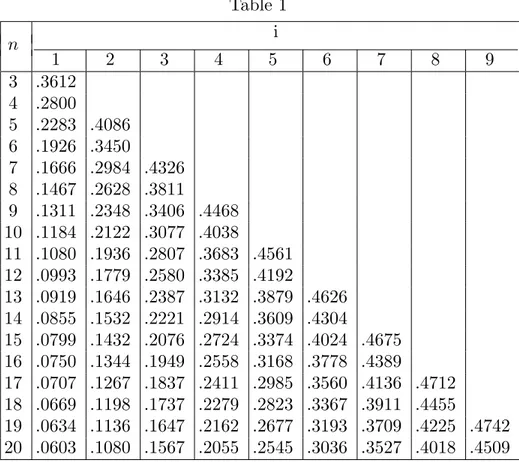
Table 1 gives us the values of qn(i) for n = 3, 4, . . . , 20. Due to the equality
vq+(i) + v1−q+ (n − i) = 1
we have q ≤ qn(i) iff 1− q ≥ qn(n − i) so that in Table 1 only the values qn(i)
for i < [n/2] are presented. Sometimes the following fact may be useful: if i∗ is optimal for estimating the qth quantile from sample of size n, then n− i∗ + 1 is optimal for estimating the (1 − q)th quantile from the same sample.
Table 1 i n 1 2 3 4 5 6 7 8 9 3 .3612 4 .2800 5 .2283 .4086 6 .1926 .3450 7 .1666 .2984 .4326 8 .1467 .2628 .3811 9 .1311 .2348 .3406 .4468 10 .1184 .2122 .3077 .4038 11 .1080 .1936 .2807 .3683 .4561 12 .0993 .1779 .2580 .3385 .4192 13 .0919 .1646 .2387 .3132 .3879 .4626 14 .0855 .1532 .2221 .2914 .3609 .4304 15 .0799 .1432 .2076 .2724 .3374 .4024 .4675 16 .0750 .1344 .1949 .2558 .3168 .3778 .4389 17 .0707 .1267 .1837 .2411 .2985 .3560 .4136 .4712 18 .0669 .1198 .1737 .2279 .2823 .3367 .3911 .4455 19 .0634 .1136 .1647 .2162 .2677 .3193 .3709 .4225 .4742 20 .0603 .1080 .1567 .2055 .2545 .3036 .3527 .4018 .4509 Examples.
1. Suppose we want to estimate the qth quantile with q = 0.3 from a sample of size n = 10. For the Bernoulli distribution we have
B(4, 10; 0.3) = 0.3504 < 1
2 < B(3, 10; 0.3) hence i0 = 3. Now q
10(3) = 0.3077 so that q < qn(i0), hence i∗ = 3.
2. For n = 8 and q = 0.75 we have B(7, 8; 0.75) = 0.3671 < 1
2 < B(6, 8; 0.75) = 0.6785 and i0 = 6. By Table 1 we have q8(6) = 1 − q8(2) = 0.7372. Now q > q8(6)
A comment.
It is interesting to observe that PMC-optimal estimator differs from that which minimizes Mean Absolute Deviation EF|F (T )−q|; the latter has been constructed
in Zieli´nski (1999). For example, to estimate the quantile of order q = 0.225, X3:10
is PMC-optimal , while X2:10 minimizes Mean Absolute Deviation.
Acknowledgment.
The research was supported by grant KBN 2 P03A 033 17.
References
Keating, J.P., Mason, R.L., and Sen, P.K. (1993) Pitman’s Measure of Closeness: A comparison of Statistical Estimators. SIAM, Philadelphia.
Keating, J.P., Mason, R.L., Rao, C.R., Sen, P.K. ed’s (1991) Pitman’s Measure of Closeness. Special Issue of Communications in Statistics - Theory and Methods, Vol. 20, Number 11
Lehmann, E.L. (1983), Theory of Point Estimation, John Wiley and Sons. Uhlmann, W. (1963), Ranggr¨ossen als Sch¨atzfuntionen, Metrika 7, 1, 23–40. Zieli´nski, R. (1999), Best equivariant nonparametric estimator of a quantile, Statis-tics and Probability Letters 45, 79–84.