Locally Weibull-Smoothed Kaplan-Meier Estimator (Wsp. Agnieszka Rossa) Preprint 599. IMPAN November 1999

(1)

LOCALLY WEIBULL-SMOOTHED KAPLAN-MEIER ESTIMATOR

Agnieszka Rossa

Dept. of Stat. Methods, University of L´od´z, Poland Rewolucji 1905, 41, L´od´z

e-mail: agrossa@krysia.uni.lodz.pl

and

Ryszard Zieli´nski

Inst. Math. Polish Acad. Sc. P.O.Box 137 Warszawa, Poland

e-mail: rziel@impan.gov.pl

ABSTRACT

Though widely used, the celebrated Kaplan-Meier estimator suffers from a disadvantage: it may happen, and in small and moderate samples it often does, that even if the difference between two consecutive times t1 and t2 (t1< t2) is

considerably large, for the values of the Kaplan-Meier estimators KM (t1) and

KM (t2) at these times we may have KM (t1) = KM (t2). Although that is a

gen-eral problem in estimating a smooth and monotone distribution function from small or moderate samples, in the context of estimating survival probabilities the disadvantage is particularly annoying. In the paper we discuss a local smooth-ing of the Kaplan-Meier estimator based on an approximation by the Weibull distribution function. It appears that Mean Square Error and Mean Absolute De-viation of the smoothed estimator is significantly smaller. Also Pitman Closeness Criterion advocates for the new version of the estimator.

AMS 1991 subject classification: Primary 62N02 secondary 62G05

Key words and phrases: Kaplan-Meier estimator, Weibull distribution, survival probability

(2)

INTRODUCTION

Let F (x), x ≥ 0, be the cumulative distribution function (CDF) of time to failure X of an item and let G(y), y ≥ 0, be the CDF of random time to censoring

Y of that item. Let T = min(X, Y ), let I(A) denote the indicator function of the

set A, and let δ = I(X ≤ Y ). Given t > 0, the problem is to estimate the ”survival probability” ¯F (t) = 1_{− F (t) from the ”incomplete” ordered sample}

(1) (T1, δ1), (T2, δ2), . . . , (Tn, δn), T1 ≤ T2 ≤ . . . , ≤ Tn

The Kaplan-Meier (1958) estimator (KM ), also called the product limit esti-mator, is defined as (2) KM (t) =          Qn i=1 1₋ δi n − i + 1 I(Ti≤t) , for t ≤ Tn _0, _{if δ} n = 1 undefined, if δn = 0 for t > Tn

In the case of ties among the Tiwe adopt the usual convention that failures (δi = 1)

precede censorings (δi = 0). By the definition, KM estimator is right-continuous.

Efron (1967) modified the estimator defining his version KM e as

(3) KM e(t) =

(

KM (t), if (t > Tn and δn = 1) or (t ≤ Tn and δ = 0)

0, otherwise

Gill (1980) proposed another modification, we shall refer to this version by KM g, as

(4) KM g(t) =

(

KM (t), if (t > Tn and δn= 1) or (t ≤ Tn)

(3)

To get some intuition concerning these versions and to illustrate our approach we shall refer to the well know example from Freireich at al. (1963) - see also Peterson (1983) or Marubini and Valsecchi (1995). The ”survival times” of 21 clinical patients were

(5) 6, 6, 6, 6∗, 7, 9∗, 10, 10∗, 11∗, 13, 16, 17∗, 19∗, 20∗, 22, 23, 25∗, 32∗, 32∗, 34∗, 35∗

where ∗ _{denotes a censored observation. Kaplan-Meier estimator for that data is}

presented in Fig. 1, and Efron and Gill versions in Fig. 2.

A disadvantage of those estimators is that in small and moderate samples it may happen, and it often does, that even if the difference between two different times t1 and t2 (t1 < t2) is considerably large, for the values of the

Kaplan-Meier estimators KM (t1) and KM (t2) at these times we may have KM (t1) = KM (t2). For example, for the above data we have KM (17) = KM (20) = 0.627

and KM (25) = KM (33) = 0.448. It is really very difficult for a statistician to explain to a practitioner why the probability to survive at least t = 25 is equal to the probability of surviving at least t = 33! The estimator we propose, denoted by

sKM , gives us sKM (17) = 0.6402, sKM (20) = 0.5824, sKM (25) = 0.5275, and sKM (33) = 0.4465 (see Fig. 3) which obviously sounds more reasonably.

Another disadvantage of the Efron and Gill estimators is that they estimate the survival probability beyond what one can reasonably conclude from the sample. It is obvious that Efron guessing will be preferable for short-tailed distributions (”a pessimistic prophet”) and Gill for the fat-tailed distributions (”an optimistic prophet”) but to reasonable choose between them one should restrict in a way the original nonparametric model. For that reason we confine ourselves to the original Kaplan-Meier version (2).

LOCAL WEIBULL SMOOTHING

Kaplan-Meier estimator is adequate for the nonparametric statistical model in which the only assumptions concerning possible distributions of life time are their continuity and strict monotonicity. There are some well known representatives of that family of distributions:

(4)

– exponential E(λ) with probability density function PDF ∝ exp{−λt} – Weibull W (λ, α) with survival probability W (t; λ, α) = exp_{−λtα_}

– gamma Γ(α, λ) with PDF ∝ tα−1_exp{−λt})

– generalized gamma Γg(λ, α, k) with PDF ∝ tαk−1exp{−λtα}

– lognormal logN (µ, σ)

– Gompertz Gom(λ, α) with survival probability exp{λ(1 − exp(αt))} – Pareto P ar(λ, α) with survival probability (1 + λt)−α

– log-logistic logL(λ, α) with survival probability 1/(1 + λtα) – exponential-power EP (λ, α) with PDF ∝ exp{−λtα}

to mention the most popular among them (e.g. Kalbfleisch and Prentice 1980, Klein et al. 1990). Here ”∝ means as usually ”proportional to”.

It is obvious that on a sufficiently short interval on the real half-line each of them my be considered as a reasonably good approximation of any CDF from the nonparametric family under consideration. We have chosen the Weibull tail

W (t; λ, α) = exp{−λtα} mainly because that gives us a simple algorithm of

calcu-lating the estimator: it is enough to perform logarithmic transformations of data and apply the standard estimating procedure for A and B in the simple regression model y = Ax + B.

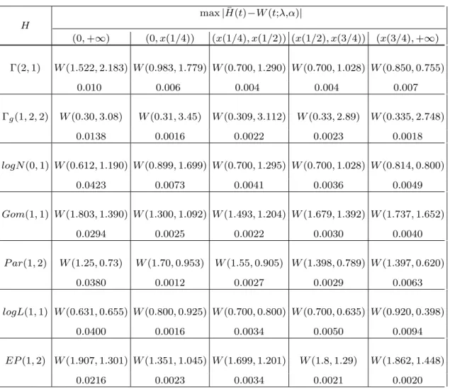
On the other hand, the Weibull family {exp{−λtα_{}, λ > 0, α > 0} of tails}

appears to be sufficiently flexible to fit all typical survival distributions. E.g. the maximal (for t > 0) difference between survival probabilities under gamma Γ(2, 1) distribution and that under Weibull W (1.522, 2.183) distribution is not greater than 0.010 (see Tab. 1).

Having the local approximation in mind we proceed as follows. Let M > 1 be a positive integer and, for a given ”typical” survival distribution H, divide the positive half-line into M disjoint intervals I(j) = [x((j − 1)/M), x(j/M)),

(5)

the distribution H. Let, for a fixed λ and α,

mj(q) = max

t∈I(j)|H(t) − W (t; λ, α)|

It is obvious that, for a given H and ε > 0, one can find M > 1, and for every

j = 1, 2, . . . , q, one can find λ and α, such that mj(q) < ε, j = 1, 2, . . . , q. Tab.1

gives us the values mj(4), j = 1, 2, 3, 4, for a set of representatives H. It appears

that if ε = 0.01 then M = 4 is enough large to ensure the local approximation within the error of ε.

If we are interested in estimating the survival probability P {X > t} for a given t, there are two possibilities to smooth an empirical survival function (ESF) ”locally”. We may choose a ”small” positive number h > 0 and approximate ESF by Weibull survival function on the interval (t − h/2, t + h/2) (”a fixed window width”). Or we may fix an integer m < n and approximate ESF on a random closed interval [Tw, Tw+m−1] which contains m points (”neighbours” of t) with a

suitably chosen w (”a fixed number of neighbours”). We prefer latter. THE ESTIMATOR

Let N_{− 1 be the number of distinct elements of the sample (1) in which}

δi= 1, i < n, and let i1, i2, . . . , iN−1 be indexes of those elements. Let T00 = 0 and

define T_j0 = Tij, TN0 = Tn. Then KM (T00) = 1 and KM (t), t < Tn, has jumps at

points T_j0_{, j = 1, 2, . . . , N − 1, and only at these points. If δ}n = 1, then also t = Tn

is a point of a jump of KM . We shall write Kaplan-Meier estimator in the form of the sequence of pairs (T0

j, KMj0), j = 1, 2, . . . , N ), where (6) KM_j0 =              KM (T0 j−1) + KM (Tj0) 2 , if j = 1, 2, . . . , N − 1 ( KM (Tn)/2 for δn = 1 KM (Tn) for δn = 0 , if j = N

Suppose we want to estimate survival probability P {X > t} at a point t. If

t > Tn and δn = 0, our estimator, like the original Kaplan-Meier estimator (2), is

(6)

First, choose ε > 0 as a satisfactory level of the error of local approximation of a survival probability by a Weibull tail and find M (see previous Section). Choose

m = [N/M ] ”neighbours” of the point t; here [x] is the greatest integer smaller or

equal to x. Observe that to fit a Weibull tail to m points, the numbe of points m should not be smaller than 2.

If m = 2k is even, define w =        1, if t < T_k0 j − k + 1, if T_j−k+10 < . . . < T_j0 _{≤ t < T}_j+10 < . . . , < Tj+k N − m + 1, if T0 N −k+1 < t

If m = 2k + 1 is odd, find T_j0∗ such that |T_j0∗ − t| ≤ |T_j0− t|, j = 1, 2, . . . , N, and define w =      1, if j∗ _{≤ k + 1} j∗_{− k,} if k + 1 < j∗ _{≤ N − k} N − m + 1, if N − k < j∗ Take T0

w, Tw+10 , . . . , Tw+m−10 as neighbours of the point t. Then fit a Weibull tail

exp{−λtα_{} to them. To this end ”linearize the tail” by introducing auxiliary}

vari-ables

xj = log(KMj0), yj = log(− log Tj0), j = w, w + 1, . . . , w + m− 1

and estimating regression coefficients Λ and α in

y = Λ + αx

where Λ = log λ. Finally, if (ˆΛ, ˆα) are estimators of those coefficients and ˆλ =

(7)

(7) _{S(t) = exp{−ˆλtˆ}α}

Like the original Kaplan-Meier estimator KM, the smoothed estimator (7) is difficult for theoretical analysis. It is however obvious that for large n and in consequence for large N (if the probability of censoring is not growing with n), and for m = m(N ) suitably growing with m/N bounded, the estimator S(t) will behave like KM. In an asymptotic setup one can hardly expect new interesting results.

In small and moderate samples the smoothed estimator may considerably differ from the original one, in such situations however general theoretical conclusions seem to be impossible. Simulation studies (next Section) demonstrates that the proposed smoothing really improve estimation.

A SIMULATION STUDY

To compare estimators on a given set of r time-points t1, t2, . . . , tr we decided

to choose points of the form tj = xqj(H) = H−1(qj) with fixed q1, q2, . . . , qr rather than with fixed t1, t2, . . . , tr because whatever the parent distribution H

the estimators at a given point xq(H) always estimate the value q. For example,

if r = 3 and q1 = 0.25, q2 = 0.5, q3 = 0.75, when studying the behaviour of

our estimators under the exponential distribution with PDF proportional to e−t

we observe their values at points 0.288, 0.693, 1.386 while under the lognormal

logN (0, 1) distribution at points 0.509, 1.0, 1.963. In both cases however what we

estimate are the survival probabilities equal to 0.75, 0.5, 0.25, respectively.

In all simulation studies presented below, due to our numerical experiments, we decided to choose m = max_{{[N/M], 3}. All results presented in the tables and} figures are based on 10, 000 simulations.

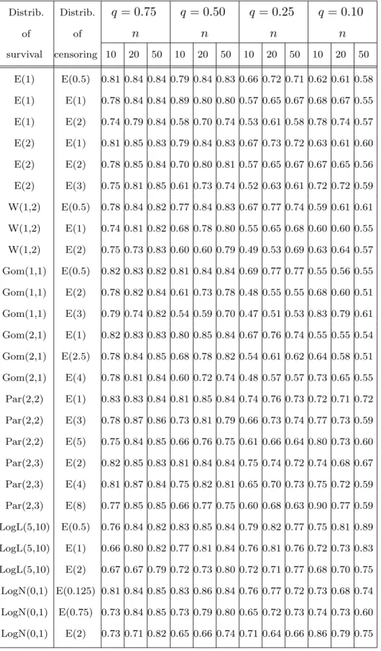
Let M SEKM(q, F, G) denote the mean square error of the Kaplan-Meier

es-timator at the point t = xq(F ) if the sample comes from the distribution F

and G is the censoring distribution. Similar notation M SEsKM(q, F, G) we

(8)

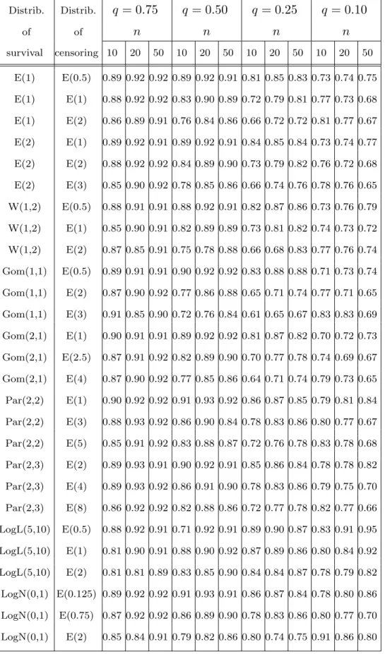
M ADKM(q, F, G) denotes the mean absolute deviation of the Kaplan-Meier

esti-mator, etc.

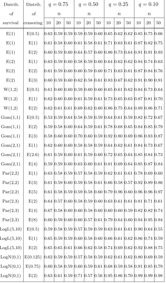
Let P CC(q, F, G) denote the Pitman Closeness Criterion (see Keating et al. 1993) for both estimators at the point t = xq(F ) if F is the survival distribution

and :

P CC(q, F, G) = PF,G{|sKM(t) − q)| ≤ |KM(t) − q)|}

If P CC(q, F, G) > 0.5 then sKM prevails in the sense that the absolute error of this estimator is smaller than that of KM more often than it is larger.

Table 2 gives us ratios M SEsKM(q, F, G)

M SEKM(q, F, G)

for some survival and censoring distributions. Table 3 gives us those values for M AD, and Table 4 the values of

P CC.

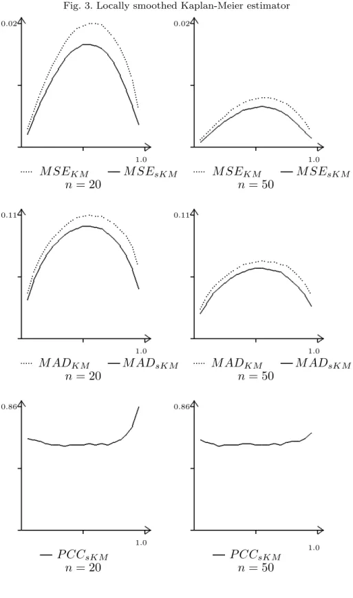
Fig. 4 exhibits M SEsKM(q, F, G), M ADKM(q, F, G)), and P CC at the whole

range of q ∈ (0, 1) for the case where the samples of size 20 or 50, respectively, come for the Weibull F = W (1, 2) distribution and censoring is exponential G = E(2). The results presented in Fig. 4 are typical for all the results we obtained under other pairs (F, G).

ADDITIONAL COMMENTS

1. Our simulations suggest that the bias of sKM is smaller than that of KM but we were not able to find a regularity in that. Whatever however the bias and the variance, with respect to M SE and M AD smoothed sKM is better than the original KM .

2. Sufficiently far to the right, the original Kaplan-Meier estimator in all simu-lations gives the values zero. It follows that ”practically”, for large t, it’s variance is equal to zero. That of course is not the case for sKM .

3. In our simulations we were also interested in M SE and other characteristics of the estimators under consideration if there is no censoring. For every q ∈ (0, 1) the Kaplan-Meier estimator is then unbiased and is variance at the point xq(F ) is

(9)

equal to q(1_{− q)/n. It is interesting to observe (Fig. 5) that sometimes censoring} can improve M SE. On a paradox of this kind see Cs¨org¨o et al. (1998).

4. A disadvantage of the smoothed estimator consists in that it may happen, and sometime it does (see Fig. 6), that sKM (t1) < sKM (t2) though t1 < t2. It

may happen if t1 has a value close to the upper bound of the interval of those t,

which are estimated by smoothing the points at T_w0, T_w+10 , . . . and t2 is close to

the lower bound of the interval of those t, which are estimated by smoothing the points at T0

w+1, Tw+20 , . . .. The problem is that what we propose is not a global

smoothing of the Kaplan-Meier estimator, but a local smoothing for estimating survival probability at a given point t, for each t separately. A kind of adjustment of estimators at two adjacent points is however needed but as yet we do not how to approach the problem.

(10)

REFERENCES

Cs¨org¨o, S. and Faraway, J.J. (1998). The paradoxical nature of the proportional hazards model of random censorship. Statistics 31, 67-78

Efron, B. (1967). The two-sample problem with censored data. Proceedings of the

Fifth Berkeley Symposium on Mathematical Statistics and Probability 4, 831–852

Freireich, E.O. et al. (1963). The effect of 6-mercaptopurine on the duration of steroid-induced remission in acute leukemia: a model for evaluation of other po-tentially useful therapy. Blood 21, 699–716

Gill, R.D. (1980). Censoring and Stochastic Integrals,. Mathematical Centre Tract No. 124, Amsterdam: Mathematisch Centrum.

Kalbfleisch, J.D. and Prentice, R.L. (1980). The stastistical analysis of failur time

data. Wiley

Kaplan, E.L. and Meier, P. (1958). Nonparametric estimation from incomplete observations. Journal of the American Statistical Association, 53, 457–481.

Keating, J.P., Mason, R.L, and Sen, P.K. (1993). Pitman’s Measure of Closeness: A comparison of Statistical Estimators SIAM Philadelphia

Klein, J.P., Lee, S.C. and Moeschberger, M.L. (1990). A partially parametric es-timator of survival in the presence of randomly censored data. Biometrics, 46, 795–811.

Marubini, E. and Valsecchi, M.G. (1995). Analysing Survival Data from Clinical

Trials and Observational Studies, Wiley

Peterson, A.V. (1983). Kaplan-Meier estimator. In Encyclopedia of Statistical

(11)

Tab. 1 max | ¯H(t)−W (t;λ,α)| H (0, +∞) (0, x(1/4)) (x(1/4), x(1/2)) (x(1/2), x(3/4)) (x(3/4), +∞) Γ(2, 1) W (1.522, 2.183) W (0.983, 1.779) W (0.700, 1.290) W (0.700, 1.028) W (0.850, 0.755) 0.010 0.006 0.004 0.004 0.007 Γg(1, 2, 2) W (0.30, 3.08) W (0.31, 3.45) W (0.309, 3.112) W (0.33, 2.89) W (0.335, 2.748) 0.0138 0.0016 0.0022 0.0023 0.0018 logN (0, 1) W (0.612, 1.190) W (0.899, 1.699) W (0.700, 1.295) W (0.700, 1.028) W (0.814, 0.800) 0.0423 0.0073 0.0041 0.0036 0.0049 Gom(1, 1) W (1.803, 1.390) W (1.300, 1.092) W (1.493, 1.204) W (1.679, 1.392) W (1.737, 1.652) 0.0294 0.0025 0.0022 0.0030 0.0040 P ar(1, 2) W (1.25, 0.73) W (1.70, 0.953) W (1.55, 0.905) W (1.398, 0.789) W (1.397, 0.620) 0.0380 0.0012 0.0027 0.0029 0.0063 logL(1, 1) W (0.631, 0.655) W (0.800, 0.925) W (0.700, 0.800) W (0.700, 0.635) W (0.920, 0.398) 0.0400 0.0016 0.0034 0.0050 0.0094 EP (1, 2) W (1.907, 1.301) W (1.351, 1.045) W (1.699, 1.201) W (1.8, 1.29) W (1.862, 1.448)

(12)

Tab. 2 Distrib. Distrib. q = 0.75 q = 0.50 q = 0.25 q = 0.10 of of n n n n survival censoring 10 20 50 10 20 50 10 20 50 10 20 50 E(1) E(0.5) 0.81 0.84 0.84 0.79 0.84 0.83 0.66 0.72 0.71 0.62 0.61 0.58 E(1) E(1) 0.78 0.84 0.84 0.89 0.80 0.80 0.57 0.65 0.67 0.68 0.67 0.55 E(1) E(2) 0.74 0.79 0.84 0.58 0.70 0.74 0.53 0.61 0.58 0.78 0.74 0.57 E(2) E(1) 0.81 0.85 0.83 0.79 0.84 0.83 0.67 0.73 0.72 0.63 0.61 0.60 E(2) E(2) 0.78 0.85 0.84 0.70 0.80 0.81 0.57 0.65 0.67 0.67 0.65 0.56 E(2) E(3) 0.75 0.81 0.85 0.61 0.73 0.74 0.52 0.63 0.61 0.72 0.72 0.59 W(1,2) E(0.5) 0.78 0.84 0.82 0.77 0.84 0.83 0.67 0.77 0.74 0.59 0.61 0.61 W(1,2) E(1) 0.74 0.81 0.82 0.68 0.78 0.80 0.55 0.65 0.68 0.60 0.60 0.55 W(1,2) E(2) 0.75 0.73 0.83 0.60 0.60 0.79 0.49 0.53 0.69 0.63 0.64 0.57 Gom(1,1) E(0.5) 0.82 0.83 0.82 0.81 0.84 0.84 0.69 0.77 0.77 0.55 0.56 0.55 Gom(1,1) E(2) 0.78 0.82 0.84 0.61 0.73 0.78 0.48 0.55 0.55 0.68 0.60 0.51 Gom(1,1) E(3) 0.79 0.74 0.82 0.54 0.59 0.70 0.47 0.51 0.53 0.83 0.79 0.61 Gom(2,1) E(1) 0.82 0.83 0.83 0.80 0.85 0.84 0.67 0.76 0.74 0.55 0.55 0.54 Gom(2,1) E(2.5) 0.78 0.84 0.85 0.68 0.78 0.82 0.54 0.61 0.62 0.64 0.58 0.51 Gom(2,1) E(4) 0.78 0.81 0.84 0.60 0.72 0.74 0.48 0.57 0.57 0.73 0.65 0.55 Par(2,2) E(1) 0.83 0.83 0.84 0.81 0.85 0.84 0.74 0.76 0.73 0.72 0.71 0.72 Par(2,2) E(3) 0.78 0.87 0.86 0.73 0.81 0.79 0.66 0.73 0.74 0.77 0.73 0.59 Par(2,2) E(5) 0.75 0.84 0.85 0.66 0.76 0.75 0.61 0.66 0.64 0.80 0.73 0.60 Par(2,3) E(2) 0.82 0.85 0.83 0.81 0.84 0.84 0.75 0.74 0.72 0.74 0.68 0.67 Par(2,3) E(4) 0.81 0.87 0.84 0.75 0.82 0.81 0.65 0.70 0.73 0.75 0.72 0.59 Par(2,3) E(8) 0.77 0.85 0.85 0.66 0.77 0.75 0.60 0.68 0.63 0.90 0.77 0.59 LogL(5,10) E(0.5) 0.76 0.84 0.82 0.83 0.85 0.84 0.79 0.82 0.77 0.75 0.81 0.89 LogL(5,10) E(1) 0.66 0.80 0.82 0.77 0.81 0.84 0.76 0.81 0.76 0.72 0.73 0.83 LogL(5,10) E(2) 0.67 0.67 0.79 0.72 0.73 0.80 0.72 0.71 0.77 0.68 0.70 0.75 LogN(0,1) E(0.125) 0.81 0.84 0.85 0.83 0.86 0.84 0.76 0.77 0.72 0.73 0.68 0.74 LogN(0,1) E(0.75) 0.73 0.84 0.85 0.73 0.79 0.80 0.65 0.72 0.73 0.74 0.73 0.60

(13)

(14)

(15)

0.0 0.5 1.0

6 7 10 13 16 22 23 35

Fig.1 The Kaplan-Meier estimator KM

0.0 0.5 1.0 6 7 10 13 16 22 23 35 KM e KM g

Fig.2 The Efron’s and Gill’s versions of the Kaplan-Meier estimator

1.0

0.64 •

0.58 •

0.53 •

(16)

Fig. 3. Locally smoothed Kaplan-Meier estimator 0.86 1.0 P CCsKM n = 20 0.86 1.0 P CCsKM n = 50 0.11 1.0 ... ... ... ... ... ... ... .. ... .... .... .... .... ... _{M AD}_KM _{M AD}_sKM n = 20 0.11 1.0 ... ... ... ... ..._.... ..._... ... _{M AD}_KM _{M AD}_sKM n = 50 0.02 1.0 ... ... ... ... ... ... ... ... .... .... .... ...._... .... ...._.. ... _{M SE}_KM _{M SE}_sKM n = 20 0.02 1.0 ... ... ... . . ... .... ...._.. ... _{M SE}_KM _{M SE}_sKM n = 50

Fig. 4 SimulatedM SE,M ADandP CC for the Kaplan-Meier estimator

(17)

0.00 0.01 0.1 0.2 0.3 0.4 0.5 0.6 0.7 0.8 0.9 1.0 .. .. .. .. .. .. .. ... . .. . . .. . . .. . . .. . . . . .. . . . . . . . . . . . . . . . . . . . ._. ._. ._. ._. . . . ._. . . . .. .. .. .. .. .. .. .. . .. ... . .. . . .. . . .. . . .. . . . . _{. .} . . ._{. .} . . . . ._. ._. . . . ._. ._. . . . . . . . . . . . _{M SE}_EDF . . . _{M SE}_KM M SEsKM

Fig.5. SimulatedM SE of the Kaplan-Meier estimator and the smoothed estimator

(18)

Sample size n=20. 6 7 10 13 16 22 23 35 0 0.25 0.50 0.75 1.00 _... ..._... ..._... ..._... ..._... ..._... ..._... ... ..._... ..._... ..._... ..._... ..._...