Optimization of logistic motor transport networks with application of propositional calculus laws

(1)

OPTIMIZATION OF LOGISTIC MOTOR TRANSPORT

NETWORKS WITH APPLICATION

OF PROPOSITIONAL CALCULUS LAWS

Andrzej A. Czajkowski, Józef Frąś, Mathias Schlegel

and Norbert Kanswohl****

* Faculty of Automotive Systems, Higher School of Technology and Economics in Szczecin, Klonowica 14, 71-244, Szczecin, Poland, Email:czajko2@o2.pl ** Faculty of Engineering Management, Poznan University of Technology, Strzelecka 11,

60-965, Poznan, Poland, E-mail: jozef.fras@put.poznan.pl

*** Faculty of Agricultural and Enviromental Sciences, University of Rostock, Justus-von-Liebig-Weg 6, 18051, Rostock, Germany, E-mail: mathias.schlegel@uni-rostock.de **** Faculty of Agricultural and Enviromental Sciences, University of Rostock, Justus-von-Liebig-Weg 6, 18051, Rostock, Germany, E-mail: norbert.kanswohl@uni-rostock.de

Abstract Some proposition of mathematical logic application for optimization of logistic nets describing motor transport has been presented in this paper. Some algorithm for optimization steps has been proposed in the article. In presented example has been elaborated some optimization of logistic net for motor transport. The optimized logistics network for motor transport significantly improves reliability and contributes to the economical use of the vehicle.

Paper type: Research Paper Published online: 15 April 2019

Vol. 9, No. 2, pp. 65–76

DOI: 10.21008/j.2083-4950.2019.9.2.1 ISSN 2083-4942 (Print)

ISSN 2083-4950 (Online)

(2)

1. INTRODUCTION

A logistics network is a group of events describing the modelling of motor transport. By the symbol T we will denote a certain event that occurs in the assumptions of the transport logistics. Operation of the logistics network is based on the appearance or non-appearance of the event in points in the network, which is interpreted as an admission by a variable T the value of 1 (there is a transport) or 0 (there is not a transport). Propositional calculus can be used to optimize logistics networks which describe some transport. Logistics network is based on three main elements: summing element (), product element () and negating element (). Symbols ,  and  mean the conjunctions “or”, “and” and “not” (Fig. 1).

Fig. 1 Basic input transports T1, T2, T and output transports X, Y, Z of logistics transport

network

Properties 1–2. (Laws of commutative and connection of alternatives) (Grzegorczyk, 1969; Majewski, 2003; Rutkowski, 1978)

For any transports T1, T2:

Properties 3–4. (Lows of commutative and connection of conjunction) (Grzegorczyk, 1969; Majewski, 2003; Rutkowski, 1978)

For any transports T1, T2:

Properties 5–6.

[Laws of separation of conjunctions (alternatives) to the alternatives (conjunction)] (Grzegorczyk, 1969; Majewski, 2003; Rutkowski, 1978)

(3)

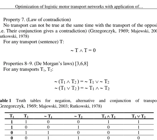
Property 7. (Law of contradiction)

No transport can not be true at the same time with the transport of the opposite (i.e. Their conjunction gives a contradiction) (Grzegorczyk, 1969; Majewski, 2003; Rutkowski, 1978)

For any transport (sentence) T:

Properties 8–9. (De Morgan’s laws) [3,6,8] For any transports T1, T2:

Table 1 Truth tables for negation, alternative and conjunction of transports

(Grzegorczyk, 1969; Majewski, 2003; Rutkowski, 1978)

T1 T2  T1  T2 T1 T2 T1 T2

1 1 0 0 1 1

1 0 0 1 0 1

0 1 1 0 0 1

0 0 1 1 0 0

The existence or non-existence of T1 and T2 transports for basic logic systems

can be presented in the corresponding table (i.e. for negation, conjunction and alternatives of transports) (Tab. 1).

2. MODELLING OF MOTOR TRANSPORT CONDITIONS

In modelling of a motor transport network, some selected laws of the propositional calculus have been used. Taking into account the modelling of transport, its analytical description, the optimization of patterns and the correctness of the analysed schemes, the authors propose to adopt the scheme of steps (Fig. 2).

(4)

Fig. 2 The steps modelling and optimization of logistics networks

The suggested scheme of action can be used equally well to describe the flow patterns in other logistics networks. In the above diagram, the authors propose the use of an analytical method to carry out the optimization process. In addition, numerical proofs of the correctness of the optimization process are shown. Numeric programs, such as Mathematica, MS-Excel and MathCAD, are used in numerical proofs. It should be noted, however, that there are computer programs that themselves carry out optimization without the need for an analytical and numerical method.

3. OPTIMIZATION OF SELECTED LOGISTIC NETS DESCRIBING

MOTOR TRANSPORT

Step 1:

Let us suppose T1, T2, T3 and T4 mean some transports of apples. These

transports T1, T2, T3 and T4 are realized according to the following assumption:

[are not realized (transport T1 or transport T3) and is realized the transport T2] or

{[(is not realized transport T3 and is realized transport T2) or is realized

(5)

Step 2:

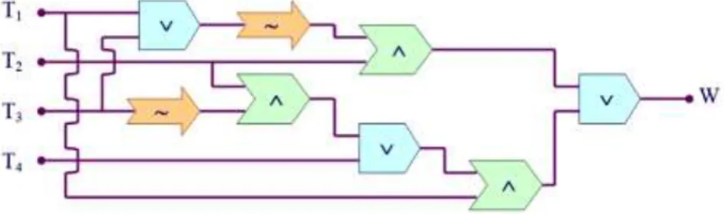
Based on that assumption it is possible to build a logistics network LN-A (Fig. 3). The transports T1, T2, T3 and T4 – among the other selections – there are

some portion of apples. Point W of the logistics network describes a target of delivery transports. To delivery point W by connections according with the logistics network NL-A may reach the species of apples from any transport T1, T2,

T3 and T4.

It should be optimized the logistics network LN-A to apply the assumption, propositional calculus laws in order to reduce discussed transport logistics network. The logistics network LN-A before optimisation has 8 logic gates for transports T1,

T2, T3, T4 and the target point W (Fig. 3).

Fig. 3 Logistics network LN-A with 8 logic gates for transports T1, T2, T3, T4 and the target

point W before optimisation Step 3:

Logistics network LN-A formed according to the scheme in Fig. 2 describes the formula:

Step 4:

Property 10. (Formula to proof)

For any of the three elements T1, T2, T3 of logistics network:

Proof:

Using de Morgan law and distributive law of conjunction, to the left side of the formula (11) we get:

(6)

In the formula (12) we apply the associative law of conjunction, and then we have:

Taking into account in the formula (13) two times the associative law of conjunction we have:

Using the distributive law of alternative in the formula (14) we get:

Using the law of contradiction in the formula (15) we get:

which is equivalent to the right side of equation (11), and also completes the proof of the property 10.

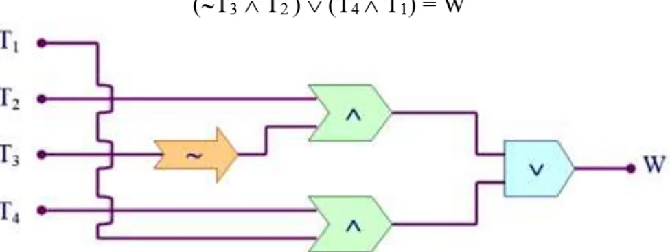
Step 5:

Optimized logistics network LN-B can be described by the following formula:

Fig. 4 Logistic network LN-B with 4 logic gates for transports T1, T2, T3, T4 and the target

(7)

Step 7:

Let us perform proofs of formula (11) for schemas LN-A and LN-B by using numerical programs Mathematica, MS-Excel and MathCAD.

Proof of formula (11) by using Mathematica program

In Mathematica we have symbol ! for negation, || for alternative, && for conjunction.

Table 2 Mathematica program for the formula (10) (Abel, 1993; Grzymkowski, Kapusta

& Słota, 1994; Trott, 2006)

Mathematica for formula: [(T1T3)T2 ]{[(T3T2)T4]T1} Results: In[1]:= T1=False;T2=False;T3=False;T4=False; (!(T1||T3)&&T2)||(((!T3&&T2)||T4)&&T1) T1=False;T2=False;T3=False;T4=True; (!(T1||T3)&&T2)||(((!T3&&T2)||T4)&&T1) T1=False;T2=False;T3=True;T4=False; (!(T1||T3)&&T2)||(((!T3&&T2)||T4)&&T1) T1=False;T2=False;T3=True;T4=True; (!(T1||T3)&&T2)||(((!T3&&T2)||T4)&&T1) T1=False;T2=True;T3=False;T4=False; (!(T1||T3)&&T2)||(((!T3&&T2)||T4)&&T1) T1=False;T2=True;T3=False;T4=True; (!(T1||T3)&&T2)||(((!T3&&T2)||T4)&&T1) T1=False;T2=True;T3=True;T4=False; (!(T1||T3)&&T2)||(((!T3&&T2)||T4)&&T1) T1=False;T2=True;T3=True;T4=True; (!(T1||T3)&&T2)||(((!T3&&T2)||T4)&&T1) T1=True;T2=False;T3=False;T4=False; (!(T1||T3)&&T2)||(((!T3&&T2)||T4)&&T1) T1=True;T2=False;T3=False;T4=True; (!(T1||T3)&&T2)||(((!T3&&T2)||T4)&&T1) T1=True;T2=False;T3=True;T4=False; (!(T1||T3)&&T2)||(((!T3&&T2)||T4)&&T1) T1=True;T2=False;T3=True;T4=True; (!(T1||T3)&&T2)||(((!T3&&T2)||T4)&&T1) T1=True;T2=True;T3=False;T4=False; (!(T1||T3)&&T2)||(((!T3&&T2)||T4)&&T1) T1=True;T2=True;T3=False;T4=True; (!(T1||T3)&&T2)||(((!T3&&T2)||T4)&&T1) T1=True;T2=True;T3=True;T4=False; (!(T1||T3)&&T2)||(((!T3&&T2)||T4)&&T1) T1=True;T2=True;T3=True;T4=True; (!(T1||T3)&&T2)||(((!T3&&T2)||T4)&&T1) Out[1]= False Out[2]= False Out[3]= False Out[4]= False Out[5]= True Out[6]= True Out[7]= False Out[8]= False Out[9]= False Out[10]= True Out[11]= False Out[12]= True Out[13]= True Out[14]= True Out[15]= False Out[16]= True

(8)

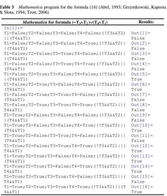
Table 3 Mathematica program for the formula (16) (Abel, 1993; Grzymkowski, Kapusta

& Słota, 1994; Trott, 2006)

Mathematica for formula (T3T2 )(T4T1) Results:

In[1]:= T1=False;T2=False;T3=False;T4=False;(!T3&&T2) ||(T4&&T1) T1=False;T2=False;T3=False;T4=True;(!T3&&T2)| |(T4&&T1) T1=False;T2=False;T3=True;T4=False;(!T3&&T2)| |(T4&&T1) T1=False;T2=False;T3=True;T4=True;(!T3&&T2)|| (T4&&T1) T1=False;T2=True;T3=False;T4=False;(!T3&&T2)| |(T4&&T1) T1=False;T2=True;T3=False;T4=True;(!T3&&T2)|| (T4&&T1) T1=False;T2=True;T3=True;T4=False;(!T3&&T2)|| (T4&&T1) T1=False;T2=True;T3=True;T4=True;(!T3&&T2)||( T4&&T1) T1=True;T2=False;T3=False;T4=False;(!T3&&T2)| |(T4&&T1) T1=True;T2=False;T3=False;T4=True;(!T3&&T2)|| (T4&&T1) T1=True;T2=False;T3=True;T4=False;(!T3&&T2)|| (T4&&T1) T1=True;T2=False;T3=True;T4=True;(!T3&&T2)||( T4&&T1) T1=True;T2=True;T3=False;T4=False;(!T3&&T2)|| (T4&&T1) T1=True;T2=True;T3=False;T4=True;(!T3&&T2)||( T4&&T1) T1=True;T2=True;T3=True;T4=False;(!T3&&T2)||( T4&&T1) T1=True;T2=True;T3=True;T4=True;(!T3&&T2)||(T 4&&T1) Out[1]= False Out[2]= False Out[3]= False Out[4]= False Out[5]= True Out[6]= True Out[7]= False Out[8]= False Out[9]= False Out[10]= True Out[11]= False Out[12]= True Out[13]= True Out[14]= True Out[15]= False Out[16]= True

The both sides of equation (11) are equivalent. That completes the proof of property 10.

Proof of formula (11) by using MS-Excel program In MS-Excel we have:

operation =JEŻELI(NIE(X)=PRAWDA;1;0) for negation,

operation =JEŻELI(LUB(X1;X2)=PRAWDA;1;0) for alternative, operation =JEŻELI(ORAZ(X1;X2)=PRAWDA;1;0) for conjunction,

(9)

operation =JEŻELI(ORAZ(JEŻELI(X1<=X2;1;0);JEŻELI(X2<=X1;1;0));1,0) for equivalence.

where X, X1, X2 mean some realisation of transports which in MS-Excel program have the values 1 for realized transport and 0 for non-realized transport.

Table 5 MS-Excel program for the formula (10) (Gonet, 2010; Smogur, 2008; University

of Cape Town, 2013) A B T1 T2 T3 T4 T1T3 (T1T3) (T1T3) T2 T3 T3T2 (T3T2) T4 [(T3T2) T4] T1 AB 0 0 0 0 0 1 0 1 0 0 0 0 0 0 0 1 0 1 0 1 0 1 0 0 0 0 1 0 1 0 0 0 0 0 0 0 0 0 1 1 1 0 0 0 0 1 0 0 0 1 0 0 0 1 1 1 1 1 0 1 0 1 0 1 0 1 1 1 1 1 0 1 0 1 1 0 1 0 0 0 0 0 0 0 0 1 1 1 1 0 0 0 0 1 0 0 1 0 0 0 1 0 0 1 0 0 0 0 1 0 0 1 1 0 0 1 0 1 1 1 1 0 1 0 1 0 0 0 0 0 0 0 1 0 1 1 1 0 0 0 0 1 1 1 1 1 0 0 1 0 0 1 1 1 1 1 1 1 0 1 1 0 0 1 1 1 1 1 1 1 1 0 1 0 0 0 0 0 0 0 1 1 1 1 1 0 0 0 0 1 1 1

Table 6 MS-Excel program for the formula (16) (Gonet, 2010; Smogur, 2008; University

of Cape Town, 2013) T1 T2 T3 T4 T3  T3 T2 T4 T1 (T3 T2)  (T4 T1) 0 0 0 0 1 0 0 0 0 0 0 1 1 0 0 0 0 0 1 0 0 0 0 0 0 0 1 1 0 0 0 0 0 1 0 0 1 1 0 1 0 1 0 1 1 1 0 1 0 1 1 0 0 0 0 0 0 1 1 1 0 0 0 0 1 0 0 0 1 0 0 0 1 0 0 1 1 0 1 1 1 0 1 0 0 0 0 0 1 0 1 1 0 0 1 1 1 1 0 0 1 1 0 1 1 1 0 1 1 1 1 1 1 1 1 0 0 0 0 0 1 1 1 1 0 0 1 1

(10)

From comparison of the last columns in the Table 5 we see that they are identical. This fact means that the logistics networks LN-A and LN-B are equivalent. The both sides of equation (11) are equivalent. That completes the proof of property 10.

Proof of formula (11) by using MathCAD program

In MathCAD we have symbol  for negation,  for alternative,  for conjunction.

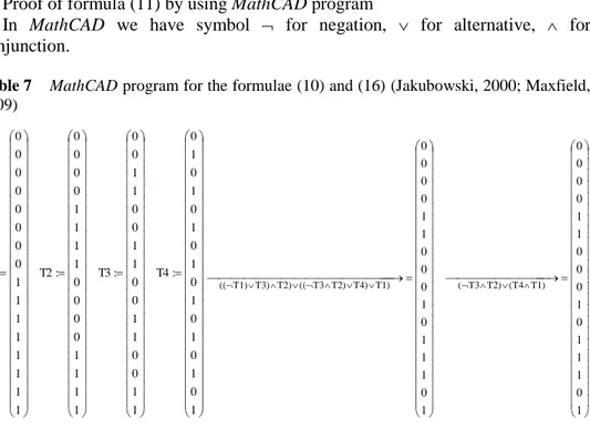
Table 7 MathCAD program for the formulae (10) and (16) (Jakubowski, 2000; Maxfield,

2009)                                                                                                                                                                                                             1 0 1 0 1 0 1 0 1 0 1 0 1 0 1 0 : T4 1 1 0 0 1 1 0 0 1 1 0 0 1 1 0 0 : T3 1 1 1 1 0 0 0 0 1 1 1 1 0 0 0 0 : T2 1 1 1 1 1 1 1 1 0 0 0 0 0 0 0 0 : T1                                                                                                                                  _ _ _ _ _ _ _ _ _ _ _ _ 1 0 1 1 1 0 1 0 0 0 1 1 0 0 0 0 1 0 1 1 1 0 1 0 0 0 1 1 0 0 0 0 T1) (T4 T2) T3 ( T1) T4) T2) T3 (( T2) T3) T1) ((

From the comparison of two vectors in the table 7 we see that they have identical values. This fact means that the logistics networks LN-A and LN-B are equivalent. The both sides of equation (11) are equivalent. That completes the proof of property 10.

The results of numerical analysis in programs MS-Excel, Mathematica and

MathCAD for the logistics networks LN-A and LN-B proof the property 10 is true.

Step 8:

We see that the transports T1, T2, T3 and T4 which have some parts of apples,

are car-ried out to the target point W by transport realization according with 7 input systems (0100), (0101), (1001), (1011), (1100), (1101) and (1111). Input system (0000) indicates that none of the four transports T1, T2, T3, T4 is not implemented.

This means that it is possible to use the optimized logistics transport networks LN-B which is described by the formula (not T3 and T2) or (T1 and T4).

(11)

4. RESULTS AND DISCUSSION

In obtained input systems (0100), (0101), (1001), (1011), (1100), (1101), (1111) we can see the following realization of transports to the target point W:

• input system (0100) means that only transport T2 is realized,

• input system (0101) means that only two transports T2 and T4 are realized,

• input system (1011) means that only three transports T1, T3 and T4 are

realized,

• input system (1101) means that only three transports T1, T2 and T4 are

realized,

• input system (1111) means that all four transports T1, T2, T3 and T4 are

realized.

The most economical transport, as to the number of trucks, is realized by the exit (1000). The most unfavourable transport, as to the number of trucks, is carried out by the exit (1111). The most effective transport, as to the number of trucks, is carried out by the exit (0101), (1001), (1100). The average effective transport of the number of trucks is carried out by the exit (1011) and (1101).

Taking into account the above-mentioned facts, it can be stated that the LN-B logistics transport network is more advantageous than the LN-A network in terms of both economics and logistics.

The most reliable gate in both logistics transport networks is the gate (1111), which means the use of transports T1, T2, T3 and T4. However, at the gate (0100)

you get the most economical transport which means the use of only one truck T2.

Both transport logistics networks LN-A and LN-B are both equivalent and reliable.

5. CONCLUSION

Motor transport systems can be describe by elements that are fundamental gates of logistics transport networks. Logistics network for transport systems can be describe by analytical formulas or graphic patterns accordance with the propositional calculus laws.

Logistics network can be optimized by using the propositional calculus laws. Optimization of logistics network describing motor transport allows to create such logistics network that is less complicated than initially described in given transport model.

Modelling the truth tables for logistics networks can be shown by both analytical method and in numerical programs Mathematica, MS-Excel and

(12)

REFERENCES

Abel M.L. (1993) Mathematica by example. Revosed Edition, AP Professional, A Division of Hardcourt Brace & Company, Boston San Diego New York London Sydney Tokyo Toronto.

Gonet M. (2010) Excel in science and technical calculations. Helion, (in Polish).

Grzegorczyk A. (1969) An outline of mathematical logic, Mathematical Library Vol. 20, PWN, Warsaw, (in Polish).

Grzymkowski R., Kapusta A. & Słota D. (1994) Mathematica – Programming and applications, Wyd. Pracowni Jacka Skalmierskiego, Gliwice (in Polish).

Jakubowski K. (2000) MathCAD Professional. Exit.

Majewski W. (2003) Logic units. Academic textbooks EIT, WNT, Warsaw, (in Polish). Maxfield B. (2009) Essential MathCAD for Engineering Science and Math ISE. Academic

Press.

Rutkowski A. (1978) Elements of mathematical logic, Little Mathematical Library Vol. 35, WSiP, Warsaw (in Polish).

Smogur Zb. (2008) Excel in engineering applications, Helion (in Polish).

Trott M. (2006) The Mathematica guide book for symbolics. Springer Science+Business Media, Inc.

University of Cape Town (2013) Introduction to MS-Excel 2007, The open textbook. Create Space Independent Publishing Platform.