THE IMPLEMENTATION OF ECONOMIC ORDER
QUANTITY FOR REDUCING INVENTORY COST:
A CASE STUDY IN AUTOMOTIVE INDUSTRY
Mohamad Riza*, Humiras Hardi Purba** and Mukhlisin***
Master of Industrial Engineering Program, Mercu Buana University, Jln. Menteng Raya No. 29, Jakarta Pusat 10340, Indonesia
* E-mail: muhammad.riza@dsngroup.co.id ** E-mail: hardipurbaipb@gmail.com *** E-mail: mukhlisin_srg@yahoo.com
Abstract: The EOQ model is one of the oldest classic production scheduling models. The EOQ
mathematical models have been established within the scope of operations management to determine the optimal inventory level. The most widely used model is the EOQ model. This journal research uses descriptive research design. A survey was conducted on automotive components of a Japanese company in Indonesia. The company is one of the fastest growing industrial company among automotive component companies. The main products are copper materials used by the automotive industry for lamps, switches, electrical panel components two-wheeled vehicles and four-wheeled vehicles. The Japanese company seeks to meet increasing customer demand but on the other hand strive to obtain optimal inventory costs, as well as demand by parent companies in Japan for faster money turnover or otherwise known as Inventory Turnover Ratio (ITR) and must be in quantity minimum or small. This means the goods in the order must be as required.
Paper type: Case study
Published online: 19 October 2018
Vol. 8, No. 4, pp. 289–301
DOI: 10.21008/j.2083-4950.2018.8.4.1 ISSN 2083-4942 (Print)
ISSN 2083-4950 (Online)
Keywords: inventory management, economic order quantity, inventory turnover ratio
words
1. METHODOLOGY
This study adopted a descriptive research design. A survey was conducted on a Japanese company automotive component in Indonesia. The company is one of the fastest growing industrial firm among the automotive component companies. The Main products are copper material used by automotive industry for light, switch, electric panel components of two-wheeled vehicles and four-wheeled vehicles. The material is “Cooper A (C2680R-1/2H Sn0.4* 56.5)” hereinafter cal-led “Material XA1” and “Cooper B (C2600R-1/2H Sn0.8* 108)” hereinafter referred to as “Material XA2”. The company seeks to meet increasing customer demand but on the other hand strives for optimal inventory cost, also demanded by the holding company in Japan for faster turnover of money or in other words known as Inventory Turnover Ratio (ITR) and that should be in minimal or small numbers. This means that the goods in the order must be as needed (not excessive and also no shortage).
1.1. Materials
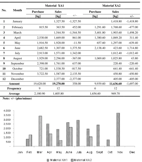
From the above data it can be concluded that both the purchasing (XA1 and XA2) materials are greater than the sales, and specifically indicate the XA1 material order is generally almost evenly distributed on every order, because of the total of 9 orders only 2 orders of distances below the average in February 2016 (815.5 kg) and October 2016 (721 kg). While the XA2 ordering material that was well below average only occurred in May 2016 (657.6 kg) of total purchasing alignment in that month.
Table 1. Two Types of Materials
Supplier Japan Koyo Company Japan Koyo Company
Materials “Cooper A (C2680R-1/2HSn0.4*56.5)” Material XA1 “Cooper B (C2600R- 1/2HSn0.8*108)” Material XA2
Based on the Figure 1 above, XA1 linear material purchase increased signify-cantly with an average of 2,180.9 kg/order, whereas for XA2 material linearly decreased with an average of 1,656.6 kg per order.
Table 2. Data of Material Purchase and Sales in 2016
No. Month
Material XA1 Material XA2
Purchase Sales +/– Purchase Sales [kg] [kg] [kg] [kg] +/– 1 January 1,327.50 -1,327.50 1,418.80 -1,418.80 2 February 815.50 363.50 452.00 1,291.60 1,768.60 -477.00 3 March 1,544.50 -1,544.50 3,401.80 1,903.60 1,498.20 4 April 2,530.00 1,669.00 861.00 1,380.60 1,069.20 311.40 5 May 1,916.50 1,928.00 -11.50 657.60 1,297.00 -639.40 6 June 2,682.50 1,307.00 1,375.50 2,138.40 423.60 1,714.80 7 July 2,913.00 1,571.00 1,342.00 1,012.40 -1,012.40 8 August 1,929.00 2,296.00 -367.00 1,069.60 1,025.80 43.80 9 September 2,398.00 1,761.00 637.00 220.40 -220.40 10 October 721.00 1,538.50 -817.50 641.40 -641.40 11 November 3,722.50 1,587.00 2,135.50 450.80 -450.80 12 December 2,377.00 -2,377.00 405.00 -405.00 Amount 19,628.00 19,270.00 358.00 9,939.60 11,636.60 -1,697.00 Frequency 9 12 6 12 Average 2,180.90 1,605.80 1,656.60 969.70 Note: +/– (plus/minus)
Fig. 1. Data of Purchasing in 2016
In general, the two materials when viewed from the EOQ side are equally less optimal, because the order frequency is relatively high, XA1 material orders nine times a year, and XA2 material has six orders in a year. This is certainly very influential on the cost of ordering, where the total cost of ordering in one year is high enough, and the impact on the total cost of inventory.
1.2. Types of Costs
a) Ordering Cost
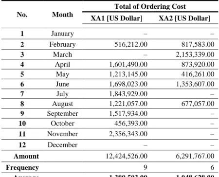
The cost of material ordering is the cost incurred in connection with material ordering i.e. the cost of material exemption from customs (customs clearance) including the cost of transportation. The length of material release is directly pro-portional to the ordering cost. The availability of original document shipment from the supplier will have an impact on the booking fee. Because without the original document shipment, material exemption process can not be done, this is because the company does not do the material release directly but hire the services of For-warder. In addition, the size of the container will also impact on the cost of booking earlier. The ordering cost in 2016 for the purchase of the material was US$633 per kilogram.
Table 3. Purchases and Sales in 2016
No. Month
Total of Ordering Cost XA1 [US Dollar] XA2 [US Dollar]
1 January – – 2 February 516,212.00 817,583.00 3 March – 2,153,339.00 4 April 1,601,490.00 873,920.00 5 May 1,213,145.00 416,261.00 6 June 1,698,023.00 1,353,607.00 7 July 1,843,929.00 – 8 August 1,221,057.00 677,057.00 9 September 1,517,934.00 – 10 October 456,393.00 – 11 November 2,356,343.00 – 12 December – – Amount 12,424,526.00 6,291,767.00 Frequency 9 6 Average 1,380,503.00 1,048,628.00
By multiplying the cost per kilogram of the monthly purchase amount (Tab. 3), we obtained the monthly cost.
b) Holding Cost
The expense of material storage is the cost incurred in relation to the storage of materials in the warehouse. In this case the company rents a warehouse from
a storage rental firm. These costs include labor costs, insurance costs, warehouse leases, electricity consumption, water use, and telephone utility.
Below is a Table 4 that provides information about the holding cost component.
Table 4. Component of Holding Cost
Holding Costs Cost in million [US Dollar] Per year
Labor Cost 48.00
Insurance Fee 222.00
Storage Rental Fee 52.00
Electricity Bill 46.00
Water Usage 1.00
Telephone Bill 5.00
Total 374.00
From the data of holding cost in the Table 4 above, the biggest cost component was insurance that must be paid annually (US$ 222 million per year) or contributed 59.35% of total holding cost (US$ 374 million per year). This should be the com-pany’s attention that meant it should be more observant to analyze the amount of material that must be stored because it will directly affect the cost of insurance, which in turn has an effect on the amount of holding costs.
1.3. Application of Economic Order Quantity (EOQ) Method
EOQ applies only when demand for a product is constant over the year and each new order is delivered in full when inventory reaches zero. There is a fixed cost for each order placed, regardless of the number of units ordered. There is also a cost for each unit held in storage, commonly known as holding cost, sometimes expres-sed as a percentage of the purchase cost of the item. Our draft is to determine the optimal number of units to order so that we minimize the total cost associated with the purchase, delivery and storage of the product.
The required parameters to the solution are the total demand for the year, the purchase cost for each item, the fixed cost to place the order and the storage cost for each item per year. Note that the number of times an order is placed will also affect the total cost, though this number can be determined from the other parameters.
1.4. Calculation of Economic Order Quantity (EOQ)
EOQ = Where:
EOQ = Economic Order Quantity S = Fixed cost per order
D = Annual demand quantity [kg] H = Annual carrying cost per unit.
Using the above formula obtained for EOQ XA1 material is as follows: EOQ =
Material EOQ XA1 = = 11,927.0 per kilogram
In the same way obtained EOQ for material XA2 by using EOQ formula,
Material EOQ XA2 =
= 8,078.0 per kilogram
Table 5. Economic Order Quantity (EOQ) Calculation Results
Descriptions Material XA1 Material XA2
Quantity of sales per period
[kilogram per year] 19,270.00 11,637.00
Cost per order [US Dollar] 1,380,503.00 1,048,628.00
Storage cost per kilogram per period
[US Dollar/kilogram/year] 374.00 374.00
EOQ within kilogram 11,927.00 8,078.00
In the Table 5 above the optimal purchase amount of material each time the message is XA1 = 11,927 kilograms and XA2 = 8,078 kilograms respectively with the purchase frequency of each material XA1 = 1.6~2 times (19,270/11,927) orders in one year, and material XA2 = 1.4~2 times (11,637/8,078) orders in one year.
Taking into account the same storage costs for material XA1 and material XA2 stored in the storage place or warehouse, material EOQ XA1 was greater than 47.6% or 3,849 kilograms compared to material XA2. This effort was done by the company to avoid the frequency of reservations that required the cost of US$ 1,380,503 per order.
1.5. Calculation of Safety Stock
Safety stock or buffer stock is a kind of inventory to anticipate uncertainty element of demand and supply. If, the safety stock is unable to anticipate the uncertainty, there will be a stock shortage. Determining the amount of safety stock can be done by comparing the sales of materials and then sought how the standard deviation. After knowing how big of standard deviation hence will be determined amount of deviation analysis. In this deviation analysis the company’s management determines how far the material is still acceptable.
Generally the tolerance limit used is 5% above the estimate and 5% below the estimate with a value of 1.65 (the Z value is obtained from the normal distribution table). Safety stock is also known as an additional quantity of an item held in the inventory in order to reduce the risk that the item will be out of stock, safety stock act as a buffer stock in case the sales are greater than planned and or the supplier is unable to deliver the additional units at the expected time.
Table 6. Computation Results of Standard Deviation from Material “XA1” in 2016
No. Purchases [kg] Deviation [kg] Quadratic
Month X (X – X) (X – X) 1 January 1,327.50 –278.30 77,469.00 2 February 363.50 –1,242.30 1,543,392.00 3 March 1,544.50 –61.30 3,762.00 4 April 1,669.00 63.20 3,990.00 5 May 1,928.00 322.20 103,791.00 6 June 1,307.00 –298.80 89,301.00 7 July 1,571.00 –34.80 1,213.00 8 August 2,296.00 690.20 476,330.00 9 September 1,761.00 155.20 24,077.00 10 October 1,538.50 –67.30 4,534.00 11 November 1,587.00 –18.80 355.00 12 December 2,377.00 771.20 594,698.00 Amount 19,270.00 0.00 2,922,913.00 Average (X) 1,605.80
Formula for calculating Standard Deviation (SD), Standard Deviation (SD) = Where:
X = Total actual material sales per period [kilogram per year] = Average of material sales in kilogram(s)
Therefore with the expression of formula above, we can obtain the standard deviation for material XA1 such as:
Standard Deviation (SD) = = = 493.5 kilograms
And then we can determine the security supplies, we know it as safety stock or buffer stock, the formula for calculating safety stock is,
Safety Stock (SS) = SD x z Where:
SD = Standard Deviation
Z = the security factor is formed on the basis of the company’s ability. Safety Stock = 493.5 × 1.65 = 814.3 kilograms
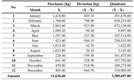
Table 7. Computation Results of Standard Deviation from Material “XA2” in 2016
No. Purchases [kg] Deviation [kg] Quadratic
Month X (X – X) (X – X) 1 January 1,418.80 449.10 201,676.00 2 February 1,768.60 798.90 638,215.00 3 March 1,903.60 933.90 872,138.00 4 April 1,069.20 99.50 9,897.00 5 May 1,297.00 327.30 107,114.00 6 June 423.60 –546.10 298,243.00 7 July 1,012.40 42.70 1,822.00 8 August 1,025.80 56.10 3,145.00 9 September 220.40 –749.30 561,475.00 10 October 641.40 –328.30 107,792.00 11 November 450.80 –518.90 269,275.00 12 December 405.00 –564.70 318,905.00 Amount 11,636.60 – 3,389,697.00 Average (X) 969.70
By applying the same formula and calculation, the standard deviation for material XA2 is obtained as:
Standard Deviation (SD) = = = 531.50 kilograms Safety Stock = SD × z = 531.5 ×1.65 = 876.90 kilograms
Then the completed calculation output of standard deviation and Safety Stock for material XA1 and material XA2 could be seen in the Table 8 such as below:
Table 8. Output of Standard Deviation and Safety Stocks for Both Materials Descriptions Material XA1 Material XA2 Standard Deviation 493.50 531.50
Safety Stock in kg 814.30 876.90
From the analysis of data above can be concluded that the greater the standard deviation that occurs then the greater safety stock that must be prepared. This shows great anticipation to the fluctuations in sales concerns.
1.6. Calculation of Reorder Point
When reordering or we call that as Reorder Point that means the time when the company has to place the ordering of the material back, so the receipt of the mate-rial ordered can be on time.
Reorder Point calculation formula (ROP), namely:
ROP = Safety Stock + (Lead time × Q) Where:
ROP = Reorder Point Lead time = Waiting time
Safety Stock = Security stock or buffer stock within kilogram(s) Q = Average material sales per month within kg per month.
ROP (XA1) = Safety Stock + (Lead time × Q) = 814,3 + (2 ×1,605) = 4,026 kg ROP (XA2) = Safety Stock + (Lead time × Q) = 876,9 + (2 × 969.7) = = 2,816.4 kg.
Table 9. Output of Reorder Point for Both Materials
Descriptions Material XA1 Material XA2 Safety stock in kg. 814.30 876.90
Lead time in month 2.00 2.00
Average sales in kg. 1,605,8.00 969.70
ROP in kilograms 4,026.00 2,816.40 From Table 9 can be concluded that for material XA1, reorder point is performed when the position of total stock is 2.5 from average sales (4,026.0 kg/1,605.0 kg), while material XA2, reorder point is performed when the position of total stock is 2.9 from average sales (2,816.0 kg/969.7 kg).
1.7. Calculation of Total Inventory Cost
To determine the total cost of raw material inventory minimally required companies using EOQ calculation. This is done for the company’s cost savings. At this cost calculation the authors make a comparison between Total Cost Inventory EOQ methods with Company Policy. The total inventory cost calculation by EOQ method is executed by applying the formula:
TIC = Where:
D = Annual demand [kg/year]
S = Cost to place a single order [US Dollar/year] H = Annual holding cost per unit [US Dollar/kg/year].
While calculation based on company policy is calculated by using formula: TIC = (Q × H) + (S × F)
Q = Average material sales per month [kg/year] S = Cost to place a single order [US Dollar/year] H = Annual holding cost per unit [US Dollar/kg/year]
F = Frequency of material purchase.
Comparison calculation of total inventory cost (Inventory Cost) by using EOQ calculation formula and company policy.
Total inventory cost for material XA1 based on EOQ:
TIC = = = US$ 4,460,775.0
Total inventory cost for material XA1 that based on company policy:
TIC = (Q ×H) + (S × F) = (1,605.8 × 374) + (1,380,503 × 9.0) =13,025,108.00 US$ b) Material XA2
Total inventory cost for material XA 2 based on EOQ:
TIC = = = US$ 3,021,166.0
Total inventory cost for material XA1 that based on company policy:
TIC = (Q × H) + (S × F) = (969.7 × 374) + (1,048,628 × 6.0) = 6,654,441.00 US$
2. FINDINGS AND DISCUSSION
Based on the below data from Table 10, it can be explained that the Total Inventory Cost (TIC) for those materials, using the method of calculating EOQ method is much cheaper, where the total cost for material XA1 is US$ 4,460,775.00 that means 190% cheaper than company policy which has the amount of US$ 13,025,108.00, and material XA2 is US$ 3,021,166.00 which explains that the cost is 120% cheaper than the figures based on company policy that shows the number of US$ 6,654,441.00 and this figure look more costly compared to EOQ method.
Table 10. Comparison of Total Inventory Costs
Descriptions Material XA1 Material XA2 TIC based on EOQ method [kg] 4,460,775.00 3,021,166.00
TIC based on company policy [kg] 13,025,108.00 6,654,441.00
From result of calculation which have been done hence can be seen comparison of material inventory between company policy and purchasing policy using Economic Order Quantity (EOQ) method, also can be seen from optimum purchase amount, purchase frequency, total cost of inventory, safety stock and when
com-pany should order back the material. So as to know which method is more efficient in the supply of materials.
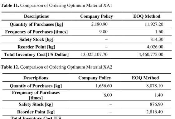
Table 11. Comparison of Ordering Optimum Material XA1
Descriptions Company Policy EOQ Method Quantity of Purchases [kg] 2,180.90 11,927.20
Frequency of Purchases [times] 9.00 1.60
Safety Stock [kg] – 814.30
Reorder Point [kg] – 4,026.00
Total Inventory Cost[US Dollar] 13,025,107.70 4,460,775.00
Table 12. Comparison of Ordering Optimum Material XA2
Descriptions Company Policy EOQ Method Quantiy of Purchases [kg] 1,656.60 8,078.10
Frequency of Purchases
[times] 6.00 1.40
Safety Stock [kg] – 876.90
Reorder Point [kg] – 2,816.40
Total Inventory Cost [US
Dollar] 6,654,441.00 3,021,165.70
From the Tables 11 and 12 above we can have some explanations that the calculation by EOQ method is much more optimal, because the total inventory cost is cheaper (EOQ cost is equal to US$ 4,460,775.00, while company policy is US$ 13,025,107.00) because the frequency of purchases more than EOQ, so the cost of the message to be large and will directly affect the total cost of inventory, and this is the same as XA2 material, the EOQ cost is US$ 3,021,165.70 and the cost obtained company policy is US$ 6,654,441.00 that explains that applying EOQ method is much better than company policy.
3. CONCLUSIONS
Inventory control and maintenance is a vital issue experienced by almost all sec-tors of the economy and this issue becomes very important topic because all orga-nizations handle inventory every day. Ignoring the importance of inventory in any organization can lead to the closure of the company, especially if the production factor is not properly managed to meet the needs or desires of the customer, the
company will stop. The inventory issue consists of a sufficient supply of goods when desired by the customer. The stock of goods must be reasonable, meaning it should not be too much or too little. Companies must be in a position to meet customer demand in terms of quantity and quality.
In general terms, inventory or stock is considered to be a major theme in mana-ging materials. Inventory Turnover Ratio (ITR) is a barometer of performance of material management functions because the ratio should be in minimal or small numbers. In commonly understood terms, inventory means the inventory of physical goods stored in the store to meet anticipated demand. However, from a material management standpoint, the other inventory definition is a usable but idle resource that has some economic value. This brings forward a paradox in the concept of inventory that is considered a necessary evil. It is necessary to have a physical stock in the system to meet anticipated demand because unavailability of materials when required will result in delays in production or projects or services provided. However, keeping inventory is not free because there is an opportunity cost to carry or hold the inventory within the organization. So, the paradox is that we need inventory, but no need to have an inventory. This is a paradoxical situation that makes inventory management a challenging area of issues in materials management. It also creates a high inventory turnover ratio as the desired performance indicator.
In inventory management, Economic Order Quantity (EOQ) is the quantity of orders that minimize the total cost of containment and booking fees. This is one of the oldest classical production scheduling models. The EOQ mathematical model has been established within the scope of operations management to determine optimal inventory levels. The assumptions made in the EOQ formulation confine the use of formulas. In practice the cost per unit of item purchase changes over time and lead time is also uncertain. This is necessary for the application of the EOQ command to keep the demand constant throughout the year that is not possible. Ordering the cost per order cannot be constant as it includes transportation costs. The booking fee is the cost to order and receive the stockpile. This includes determining how much is needed, preparing invoices, transportation costs and inspection fees. Cost shortcoming occurs when demand exceeds inventory at hand. Costs include opportunity cost to make a sale, loss of goodwill of customers, same cost of delay and similar cost.