Phase properties of elliptically polarized light propagatingin a Kerr medium with dissipation

Phase properties of elliptically polarized light propagating

in a Kerr medium with dissipation

R. Tanag

Nonlinear Optics Division, Institute of Physics, Adam Mickiewicz University, 60-780 Poznai, Poland

Ts. Gantsog

Department of Theoretical Physics, Mongolian State University, Ulan Bator 210646, Mongolia

Received April 12, 1991

The phase properties of two modes of elliptically polarized light propagating in a nonlinear Kerr medium with dissipation are studied. Exact analytical formulas for the joint phase probability distribution, the marginal phase distributions, and the individual mode phase operators, as well as the phase-difference operator expecta-tion values and variances, the phase correlaexpecta-tion funcexpecta-tion, and the expectaexpecta-tion value and the variance of the phase-difference cosine, are obtained. Some of the results are illustrated graphically to show explicitly the effect of dissipation on the evolution of the phase properties of the field.

INTRODUCTION

A quantum description of elliptically polarized light propagating in a nonlinear Kerr medium requires, in gen-eral, a two-mode approach to the problem. It was shown that such quantum effects as photon antibunching13 and squeezing4 can arise during propagation. When the light is circularly polarized, the problem can be reduced to the one-mode problem, which is equivalent to the anharmonic oscillator model. Because its simplicity permits exact so-lutions, the anharmonic oscillator model has become a testing ground for studying quantum properties of the field that is produced in a nonlinear process, and many properties of such a field have been discussed in recent years.5 2 4 For discussion of the effects associated with the propagation of elliptically polarized light in a Kerr medium a two-mode description of the field is needed. Such a description was used in the early studies 4 of the quantum field effects that appear during propagation. In those studies the Heisenberg equations of motion for the field operators were solved, and their solutions were used to calculate appropriate quantities that reveal photon antibunching or squeezing. Recently Agarwal and Puri2 5 reexamined the problem of the propagation of elliptically polarized light through a Kerr medium, discussing not only the Heisenberg equations of motion for the field opera-tors but also the evolution of the field states themselves. The polarization state of the field propagating in a Kerr medium can be described by the Stokes parameters, which are the expectation values of the corresponding Stokes op-erators when the quantum description of the field is used. Quantum fluctuations in the Stokes parameters of light propagating in a Kerr medium were discussed recently by

Tanag and Kielich.2"

The influence of dissipation on the dynamics of the anharmonic oscillator, i.e., the one-mode propagation problem, was considered by Milburn and Holmes,7 and re-cently the exact solutions of the master equation for the system were discussed. 4,17,20,21 For the two-mode case the

influence of losses and noise was discussed by HorAk and Pefina,27 whose approximate approach was based on the Heisenberg-Langevin equations of motion for the opera-tors of the two coupled nonlinear oscillaopera-tors. Recently Chaturvedi and Srinivasan,232 9 using thermodynamic field notation, found an elegant, exact solution of the mas-ter equation for a single nonlinear oscillator28 as well as for coupled nonlinear oscillators.2 9

In this paper we apply the solution of Chaturvedi and Srinivasan29 to the phase properties of elliptically polar-ized light propagating in a Kerr medium with dissipation. To describe the phase properties of the field, we use the Hermitian phase formalism introduced by Pegg and Barnett,30 3 2 which permits direct calculations of the ex-pectation values and variances of the Hermitian phase operators for the two modes of the elliptically polarized light as well as their correlations. The Pegg-Barnett phase formalism was used by Gerry3 3 and by us3 4 to study phase properties of the anharmonic oscillator without damping. We also studied3 5 the two-mode case without damping. Here we generalize our earlier results3 5 by including dissipation in the system. Exact analytical for-mulas that describe phase properties of the two-mode field propagating in a Kerr medium with dissipation are obtained and illustrated graphically to show explicitly the effect of dissipation on the evolution of the phase proper-ties of the field.

MASTER EQUATION AND ITS SOLUTION The quantum properties of elliptically polarized light propagating in an isotropic nonlinear Kerr medium can be described by the following effective interaction Hamiltonian4'35:

H = i/2hK(a+t2a+2 + aJt2a- + 4da+taita a+), (1) where a+ are the annihilation operators of the circularly right- (+) and left- (-) polarized modes, both of frequency

a, and the nonlinear coupling constant K is real and is given by

K = -r2 ]22xxyxy(c) 2h . (2) Here V denotes the quantization volume, n(o) is the linear refractive index of the medium, and Xxyxy(W) is the third-order nonlinear susceptibility tensor of the medium. The parameter d in Eq. (1) is defined by

2d = 1 + [ (3)

and describes the asymmetry of the nonlinear properties of the medium. Ritze3 has calculated this asymmetry parameter for atoms with a degenerate one-photon transi-tion, obtaining the results

d

-

{(2J

- 1) (2J + 3)/[2(2J

2

_{+ 2J + 1)] for J - J transitions}

(2J2 + 3)/[2(6J2 1)] for J - J - 1 transit

in which a+ are the amplitudes of the initial coherent states of the two modes of the field, N, = Ia± 12 are the mean number of photons, and p± are the phases of a+. The dissipation is assumed to be equal for both modes, and its value (relative to the coupling constant ) is de-scribed by A. The states

In+,

n-) = In+) In-) are the num-ber states for the plus and minus modes.

The solution, Eq. (6), is exact under the assumptions that we made here, and it is clear from Eq. (6) that it becomes a product of the solutions for individual modes if d = 0. This can happen only when the 1/2 - 1/2 transitions con-tribute to the nonlinear susceptibility of the medium. Otherwise both modes are mixed by the coupling caused by d 0. Once the solution, Eq. (6), of the master equation (5) is known, all one-time expectation values of the field operators can be found with this solution. In

ions (4) The coupling between the two modes depends crucially on

this asymmetry parameter.

Dissipation can be introduced into the system by cou-pling it to a reservoir of oscillators, which, by use of the standard techniques, leads to the following master equa-tion in the interacequa-tion picture2 9

:

at

ih-'[H,p]

+ 2(2([aip,ait]

+ [as, pait]) + yini[[ai,p],ait] }, (5) where

vj

are the damping constants and fl, are the mean numbers of thermal photons.

The exact solution to the master equation (5) was found by Chaturvedi and Srinivasan.2 9 _{In this paper we use}

their solution, restricting our considerations to the case of a zero-temperature reservoir ( = 0) and initially coher-ent state of the field. With these restrictions the solution to the master equation (5) in the number state basis reads as Pm+,m-;n+,n-(T) = (m+, mI p(T)In+, n_) = m++bn++)bm bn exp i + ) x (m+

-

n+) +

('P

+ ) (m_- -x fm+-n+;m-n- (m++n+)/2 (T)f_ (m +n-)/2(T) x exp{N+A 1 - m+-n+;m_-n_() A + [m+- n+ + 2d(m - n)] x exp{N-A +

A

I -n n m+-n+(T) (6) ~-- n + 2d(m+

-

)

where we have used the following notation:

this paper we are interested in the quantum phase proper-ties of the field propagating in a Kerr medium with dissipation.

PHASE PROPERTIES OF THE FIELD

To study phase properties of elliptically polarized light propagating in a Kerr medium, we use the new Hermitian phase formalism introduced by Pegg and Barnett.3 0 3 2

Their idea is based on introducing, for one mode of the field, a finite (s + 1)-dimensional space P spanned by the number states 0), ,...,Is). The Hermitian phase opera-tor operates on this finite space, and after all necessary expectation values have been calculated in P the value of s is allowed to tend to infinity. A complete orthonormal basis of (s + 1) states is defined in as

1 X

l1in) ( + 1)1/2 exp(ino.)ln), (10)

where

0

m o + 2rm/(s + 1) (m = 0,1,...,s). (11)

The value of 0 is arbitrary and defines a particular basis set of s + 1 mutually orthogonal phase states. The Her-mitian phase operator is defined as

'

= 2 0 m10m) (0m, I

m=0 (12)

where the subscript 0 indicates the dependence on the choice of 0. The phase states, Eq. (10), are eigenstates of the phase operator, Eq. (12), with the eigenvalues m re-stricted to lie within a phase window between 0_{o and} 0 + 2 The unitary phase operator exp(ik0,) is defined

as the exponential function of the Hermitian operator 4'. This operator, acting on the eigenstate ), gives the eigenvalue exp(iom), and it can be written a30

-32

T = Kt, A = y+/K = y-/K,

fr;n(T) = exp{-[A + i(m + 2dn)]Ir},

bn2 = exp(-N±/2)[Nn±12/(n!)112],

a. = N1/2 exp(iqp±),

exp(i4') - n) (n + 11 + exp[i(s + 1)0o] Is) (01. (13)

(8) n=o

The last term in Eq. (13) ensures that this operator is unitarity. _{The first sum reproduces the} Susskind-(9) Glogower35'37phase operator in the limit s -> .

This expectation value of the phase operator, Eq. (12), in a pure state loi) is given by

(4f4ol) =

>

Oin(0m.lJ)2'

m=O

(14)

where I(O_m1P)12 gives the probability of being in the phase state 0m). The density of phase states is (s + 1)/27r, so in the continuum limit as s tends to infinity we can write Eq. (14) as

Jq00+21r

(o)

=

OP()dO,

o

where the continuum phase distribution P(0) is intro-duced by

P(O) = lim + 1 2

S - 2r

where Om has been replaced by the continuous phase vari-able 0. Since the phase distribution function P(0) is known, all the quantum-mechanical phase expectation values can be calculated with this function in a classical-like manner. The choice of the value of 0o defines the 27r-range window of the phase values.

If the field is described by the density operator p, we have for the one-mode field, instead of Eq. (14), the relation

(+o) = Tr(p4o) = 0(0MpIOM),

and, instead of Eq. (16),

P(0) = lim 2 (0MIPI0M).

Taking into account the definition Eq. (10), we have

P(0) = lim 2 (0MIlP0M)

(16)

interests us in this paper. Proceeding along the same lines, we arrive at the following formula for the joint phase probability distribution P(O+, 0), which is symmetrized with respect to the phases o+ and So-:

P(0+,0) =

2)

₁

2 _{exp{-i[(m+ - n)(p+ + +)}

()m n +(, +

+ (m - n) (- + 0-)}Pm,m;n+,n_(0) (23) On inserting Eq. (6) into Eq. (23), we finally obtain the joint phase probability distribution for the continuous (15) phase variables 0 and 0_ describing phases of the two

modes. This gives us the following formula:

P(0+,0-) = 1 Y_ b +b +) bm-)b )m

x exp[-(A/2)(o-+ + ou-) + r(3+,8-)] x cos{6+0+ + &-0- + (/2)

[+(cr+ + 2do-_ - 1)

+ 3-(o- + 2do-+ - 1)] + A(8+,S-)}, (24) where, to shorten the notation, we have combined the summation indices: (25) (17) (18) 1 s s = lim- _ 2 exp[-i(n - k)0m]pnk(t). (19) S

2r

n=O

k=O

If we symmetrize the phase distribution with respect to a phase So by taking

0 = 4 - 7rs/(s +1) (20)

and introduce a new phase label A = m - s/2, which goes in integer steps from -s/2 to s/2, the phase distribution becomes symmetric in A, and we get

P(0) = I

> >

exp[-i(m - n)(qp + 0)]Pmn(t)- (21)

in m=O n=O

Now, all integrals over 0 are taken in the symmetric range between -or and or, and the phase distribution P(0) is

nor-malized such that

E P(0)dO = 1. (22)

All the above formulas defining phase properties of the field can easily be extended into the two-mode case that

or+ = m+ + n, 8+ = m - n, and we have defined the quantities

F(m, n) = A[Am+()n() + An-m,.(r)]

+ 7mnBm(r) + n,mB,(), A(m, n) = ., nAm+%) (T) + q nmA " (T) -A[B(+,)(T) + B " (T)], where 7mn = m + 2dn, A m)n(T) = 2NA 21 - exp(-AT)CS(j,n)]. A + 77 ,n m, n(T) = A2 + 7 2[exp-A)sin m no)] (26) (27) (28) (29) (30)

Equation (24) is the exact analytical expression that de-scribes the joint probability distribution P(0+, _), and it permits calculation of all phase expectation values by simple integrations over 0+ and 0 in the symmetrical range between -ir and 7r.

Despite the complexity of r(s+,B ) and A(3+, ), the structure of Eq. (24) is transparent. If there is no dissi-pation in the system, then A = 0, and both quantities are also equal to zero. In this case Eq. (24) coincides with our earlier result.33 Another limit is the case of no coupling between the two modes, i.e., the case d = 0, when the ex-pressions for

r(a+,

) and A(3+, ) split into sums of separate terms for the plus and minus modes, and the phase distribution P(0+, 0) can be factored into the indi-vidual mode distributions. However, either term still includes the dissipation. The one-mode case with dissi-pation was studied by us elsewhere.3 8

Because of the Poissonian weighting factors bn+(') given by Eqs. (9), the infinite sums in Eq. (24) can be evaluated numerically if the mean number of photons, N--, is not

(a)

C>

(b)

P(0+) = f

P(o+,o)dO

=- E zbm+bn++)bn-) 2r m+,n+ nf

x

(or+ + 2n-) + r(6+,O) x cos[8+0+ + (/2)8+(o-+ - 1 + 4dn-) + A(8+,0)]. ₍₃₁₎

Again, for A = 0 Eq. (31) reproduces our earlier re-sult.35 _{In fact the summation over n. can be performed,} and as a result we obtain a more compact formula for the

(a)

-7t

(c)

(b)

(d)

(c)

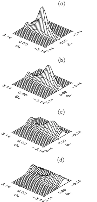
e gi.

Fig. 1. Evolution of the joint phase probability distribution func-tion P(0+,0.) for N+ = 0.25, N = 4, d = 1, and A = 0.

(a) = 0, (b) = 0.1, (c) = 0.2, (d) = 0.3.

too large. The evolution of P(0+, 0) without dissipation was studied by us previously.35

In this paper we want to show the effect of dissipation on this evolution. For ref-erence Fig. 1 shows plots of P(0+, 0 ) for A = 0 and various evolution times r. In Fig. 2 we plot P(0+, 0_) for the same times but for A = 10. As one could expect, the dissipation leads to broadening of the phase distribution, which can be clearly seen in Fig. 2. Integrating the distribution function P(0+, 0 ) over one of the phases 0+ or 0 leads to the marginal distribution P(04) or P(0+) for the individual phases. For example, we have

(d)

czo

Fig. 2. Same as Fig. 1 but for A = 10.

0.8 0.4 + 0.0

-0.4

-0.8 0.00 6.28 -7 12.56 Fig. 3. Evolution of the mean phase (+) for N = 0.25, N = 4, d = 1, A = 0 (solid curve), and A = 0.1 (curve with points superimposed).

marginal distribution P(0+), which can be written as

P(0+) = 1 + 2 E bn+)bm+) exp(-N-11 - Re[fo;nm(T)] 2 n>m - (A/2)(n +

m)

+

rF

m()) x cos{(n - m)0+ + (/2)[n(n - 1) - m(m - 1)] + N_ Im[fo;n.m(T)] + An+-m(T)}] (32) where n+) () = F(n - m, 0), A(+-) (T) = A(n - m, 0). (33) The distribution P(04) can be obtained from Eq. (32) by interchanging the indices plus and minus and taking into account that

r

(-) )

=

r( n

- m),

A- (r)

=

A(,

n

- m).

(34)

Equation (32) is quite general and contains all one-mode results obtained earlier3 3 3 538as special cases. Moreover, the structure of this formula is sufficiently simple and is reminiscent of the corresponding structure for a coher-ent state.3 2

Knowing the phase distribution, Eq. (32), permits calcu-lation of the expectation values and the variances of the Hermitian phase operators by appropriate integrations. We have, for example,

(++) = Tr(p4+) = 'p+ +

f

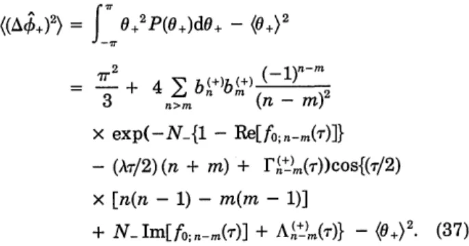
0+P(0+)dO+ = 0+ + (0+), (35) where (0+) = 0+P(0+)dO+ = 2 1 bn+)bm n- exp(-N{1 - Re[f0;nn(7)]} n>m n-m -(AT/2) (n + m) + F+)(T))sin{(7/2)[n(n - 1) - m(m - 1)] + NIm[f0;n-.m(7)] + An+)m(T)} (36) and for the variance

(( )2) = 0+2

P(0+)dO+

_ (0+)2 -7r (_l)nm

=

3 + 4

2b(+)b(+)(

)2~

3 n>m (n-r) x exp(-N-11 - Re[fo;n m(T)]} - (A/2) (n + m) + rF+) m())cos{(/2)

x

[n(n - 1) - m(m - 1)] + N Im[fo;n m(T)] + A(+) (7)} _ ( +)2. (37) Equations (36) and (37) are generalizations of our ear-lier results3" to the case with dissipation. It is to be noted that the two-mode results, even without dissipation, are periodic only if 2d is an integer or a ratio of integers. This means that periodic behavior in the two-mode case appears only for particular symmetries of the nonlinear properties of the medium. Of course, dissipation de-stroys the periodicity in any case. From Eq. (36) it is evi-dent that, because of the coupling between the two modes, there is a shift in phase of the plus mode that depends on the intensity of the minus mode. It is also seen that this shift is reduced by damping. This situation is shown in Fig. 3, where the mean phase is drawn, according to Eq. (36), for the mean number of photons N_ = 4.

The evolution of the phase variance is presented in Fig. 4, where Eq. (37) is plotted for various N_'s. For

N_ > 1, even without damping, the variance rapidly in-creases to values near v.2/3, the value for the uniformly

distributed phase. This result means that the phase of the plus mode is randomized because of the interaction with the other mode. If the evolution is periodic, how-ever, the initial values are restored after a period. Dissi-pation washed out this recurrence effect, which can be convincingly seen from Fig. 4.

When the two modes are coupled, some degree of corre-lation between them can arise during the evolution. The phase correlations can, for example, reveal themselves in the variance of the phase-difference operator of the two modes. In the Pegg-Barnett formalism the phase-difference operator is simply the phase-difference of the phase operators for the two modes, and the mean value of the phase difference is the difference of the mean values cal-culated according to Eq. (36). To calculate the variance of the phase-difference operator, we can use the following

4.0 -_ 3.5-3.

<2.5

2.0-/

1.5 -0.00 6.28 T 12.56

Fig. 4. Evolution of the phase variance ((Ak+)2) for N+ = 0.25,

d = 1, A = 0 (solid curves) and A = 0.1 (curves with points

super-imposed). The lower pair of lines is for N = 0.25 and the upper pair for N = 4.

1 .5 1.0 I C-0.5 0.0

-0.50

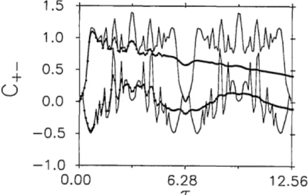
-1 .0-_ 0.00 6.28 12.56

Fig. 5. Evolution of the intermode phase correlation function

C+-(r). The upper pair of lines is for N+ = 0.25, N_ = 4, d = 1, A = 0 (solid curve), and A = 0.1 (curves with points superim-posed); the lower pair is for d = 1/2 with other values unchanged.

relation:

-+ _ )]2) = ((A^+)2) + ((A^_)2)

- 2((~++_)

-

(++)($.)).

(38)

The variances ((Ak+)2) and ((A_) 2) can be calculated ac-cording to Eq. (37), and its counterpart for the minus mode is obtained by interchanging +'s and -s. The last term, describing the correlation between the phases of the two modes, can be written as

C+ (7) = (+-)

-

NO)

= f _ 0+0_P(0+,0_)d0+d_

-

f_

0+P(0+)d0+_ 0_P(0_)d0_

= (0+0) - (0+)(0), (39)

where (0+) and (0.) are given by Eq. (36), and (0+0-)=

f

j 0+0_P(0+,0_)d0+d0_ -7z -

>

(1

b -S b+)b n++)b -b n-)(1 + -1_ x exp[-(Ar/2)(o+ + + F&5+,8-] x cos{(T/2)[6+(o+ + 2dc_ - 1)

+

8-(o-

+ 2do,+ - 1)] + A(6+,64)}, (40)

Fig. 6. Dissipation lowers the correlation between the phases that can arise during the evolution. The phase correlation function C+ (7) is an essentially two-mode phase characteristic of the field that can be calculated by means of the Pegg-Barnett phase formalism.

Except for the phases themselves and their variances, the sine and cosine functions of the individual phases as well as of the phase difference can be calculated within the Pegg-Barnett formalism. These phase characteris-tics of the field can be compared with the corresponding results of the Susskind-Glogower formalism. For calcu-lation of the sine and cosine functions of the phases, it is convenient to use the relations that hold true for physical states3 9: (exp(iro))p = (im+bSG)), (41) where 'xpimbSG) = j n) (n

+

mI n=O (42) is the Susskind-Glogower phase operator. For the phase difference we have5 (exp[im( + - k-)])p = (exp(im+)exp(-im_)), = y (In) (n ₊ ml)+ n=O

x

\(k

x

(1k +m)(ki)-)

k=0 = (e+(iMrnsG)6e-(-iMsG))p- (43) With the above relations it is easy to calculate the sine and cosine functions and their variances and compare them with the Susskind-Glogower results. The results are the following: (e4+(im0sG)) = Tr[p 6X+(im0sG)] = Y Pn+m,n-;n,n-(T) n,n-= exp[-N[{1 - Re[fo;m(7)]} - (AT/2)m + M+)(T)] x exp(i{rmp+ - (/2)m(m - 1)

-

N-Im[fo;m()] -AM+(T)}) X j b(+)bn++)mf ;O(T), n=O (44)

where the notation is the same as in Eq. (24). The prime on the summation symbol means that the terms with S+ = 0 and 5 = 0 do not enter into the sum.

Equation (40), when inserted into Eq. (39), describes the phase correlations (strictly speaking, the phase fluctua-tions correlation) that arise during the evolution of the system. If d = 0, the phase distribution P(0+, 0) factors, and C+. (r) = 0. The strength of the correlation depends crucially on the value of the asymmetry parameter d.

The highest values of the correlation are obtained for d = 1/2, which means that the minimum of the phase-difference variance, in view of Eq. (38), is obtained for d = 1/2. In Fig. 5 the correlation coefficient C(T) is plotted against for d = 1/2 and d = 1. The correspond-ing curves for the phase-difference variance are shown in

9.0 , 7.0 r-B. 1 5.0

-3.

< 3.0

Lj 1.0 -0.00 6.28 12.56

Fig. 6. Evolution of the phase-difference variance

([A(+ _ _)]2); _{the description of the curves is the same as in}

I + U) 0 in 1< 0.52 0.50 0.48

0.46

I-0.00 I-' + -'-U) 0 . 0.60 0.55 0.50 0.45 0.40 0.35 -6.28 T 12.56 0.00 6.28 12.56

f

Fig. 7. Evolution of the variance of the phase-difference cosine function ([A cos(+ - 'k)]2). The upper pair of lines is for d = 1,

and the lower pair is for d = 1/2 with A = 0 (solid curves) and A = 0.1 (curves with points superimposed). (a) N+ = 0.25 and

N = 0.25, (b) N+ = 0.25 and N = 4. The value 0.5 corresponds to the uniform phase distribution.

(cos = 1+) '/2 (exp(i++) + exp(-i4+))

= 1/2 [(/+(ik9 0)) + c.c.] = exp(-N-1 - Re[fo;j(T)]} - + r)(T)

x E b n+b+

exp(-nAT) n=0 x cos{jp+ - nT - -NIm[fo;j(T)] - A +)(T)}, (45)

(cos2 = 1/+)

'4(exp(i24+)

+ exp(-i24+) + 2) = 1/4[(`'+(i20SG)) + C.C. + 2] = 1/2 + /2 exp(-N-{1 - Re[f0;2(T)]} - At + +)(T)) i

bn+)bn++)2

n=O x exp(-nAT)cos{2p+ - (2n + 1)7 - N-Im[fo;₂(T)] - A2+)(T)}. (46) The expression for (sin A+) can be obtained from Eq. (45) by simply replacing the cosine function by the sine func-tion, and the result for (sin2 A+) can be obtained from Eq. (46) by changing the sign of the second term. Of course, the relation cos2 + + sin2 + = 1 holds in the Pegg-Barnett formalism. Equations (45) and (46) can be directly applied for calculations of variances of the phase cosine or sine. For A = 0 these formulas coincide with our earlier results.34 35

To calculate corresponding expressions for the phase difference we start with Eq. (43), which gives us

(exp[im(o+ - k_)]) = Trip Q+(imOsG)4_(-imOsG)] =

>

Pn+m,k;n,k+m(T) n,k=O = b bn+)bn++)mbk()b 1-4 nk=0 x exp[-Ar(n + k + m) +

r(m,

-m)]exp{i[m(qp+ - 'p-) - r(n - k)m(l - 2d) - A(m,-m)]}. (47)

Employing Eq. (47) in the same way as in the case of indi-vidual phases, we arrive at the expressions

(cos(P+

-4)) =

exp[-Ar +

(1, -1)]

x (+)bn++)b(-)b() exp[-Ar(n + k)] n, k=0 x cos[qp+ - So- (n - k) x (1 - 2d) - A(1,-1)], (48) (cos2(~+ - )) = 1 '/2 + /2 exp[-2Ar + r(2,-2)] x > bn+)bn++)2bk()bk(+2 exp[-Ar(n + k)] n, k=0 x cos[2%p+ - p_) - 27(n - k) x (1- 2d) - A(2,-2)]. (49)

Again, corresponding expressions for the sine function are obtained by replacing cosine with sine in Eq. (48) and by changing the sign of the second term in Eq. (49).

Equations (48) and (49) are exact analytical solutions that include damping. It is interesting to note that the cosine and sine functions of the phase difference depend merely on the difference 1 - 2d; i.e., for d = 1/2 their evolution is related only to the damping terms, and for A = 0 they remain constant. This means that the evolu-tion of the phase-difference cosine (or sine) depends cru-cially on the symmetry properties of the medium. Plots of the variance of the phase-difference cosine are pre-sented in Fig. 7. It can be clearly seen that damping smears out the oscillations and eventually drives the vari-ance to approach the value 1/2, which corresponds to a uniformly distributed phase difference. This is true even for d = 1/2, in which case there is no evolution in the ab-sence of damping.

It is interesting to compare the variances for the cosine function of the phase difference (Fig. 7) with the variance of the phase difference itself (Fig. 6). Although the reduction of the phase-difference variance for d = 1/2 is quite evident, it still shows some oscillations that are due to nonlinear dynamics of the system, while the evolu-tion of the cosine variance is due solely to the damping and is smooth. The Pegg-Barnett phase formalism makes it possible to distinguish between the two phase characteristics.

CONCLUSION

In this paper we have studied the phase properties of ellip-tically polarized light propagating in a nonlinear Kerr medium with dissipation. The new Hermitian phase

for-malism of Pegg and Barnett3 0 32 _{has been used to describe}

the phase properties of the field. The exact solution of the master equation for two coupled nonlinear oscillators, obtained recently by Chaturvedi and Srinivasan,21,9 has been applied to obtain all the expectation values, the exact analytical formulas for the joint phase probability distri-bution, marginal phase distributions, expectation values, variances of the individual mode phase operators and the phase-difference operator, and the phase correlation func-tion as well as the expectafunc-tion value and variance of the phase-difference cosine. The role of dissipation in the evolution of the phase quantities mentioned above has been discussed and illustrated graphically. As one would expect, damping smears out the quantum interference ef-fects and removes quantum periodicity from the evolution of the phase quantities. The ultimate effect of damping is always the uniform phase distribution of the vacuum state toward which the field eventually evolves. If damp-ing is not large or the evolution time is short enough, the quantum effects can still be observed, and a clear advan-tage of our exact analytical formulas is that the effect of damping can be precisely predicted.

In our present considerations we have used discrete cav-ity modes to describe the field propagating in a Kerr medium. Usually the transition to the propagation prob-lem, instead of to the cavity field probprob-lem, is made by re-placing t with - z/v. In fact, we made such a replacement in our previous study35; that is, for comparison of the present results with those of Ref. 35, one has to replace with -.

Recently the quantum theory of optical-wave propa-gation without recourse to cavity quantization was formulated.40 This approach allows one to avoid some anomalous cavity size dependences that obscured inter-pretation of the results obtained in the discrete-mode approach. The exact solution for quantum self-phase modulation has been obtained with this new approach.4

REFERENCES

1. H. H. Ritze and A. Bandilla, Opt. Commun. 29, 126 (1979). 2. R. Tanag and S. Kielich, Opt. Commun. 30, 443 (1979).

3. H. H. Ritze, Z. Phys. B 39, 353 (1980).

4. R. Tanag and S. Kielich, Opt. Commun. 45, 351 (1983); Opt. Acta 31, 81 (1984).

5. R. Tanag, in Coherence and Quantum Optics V, L. Mandel and E. Wolf, eds. (Plenum, New York, 1984), p. 645.

6. G. J. Milburn, Phys. Rev. A 33, 674 (1986).

7. G. J. Milburn and C. A. Holmes, Phys. Rev. Lett. 56, 2237 (1986).

8. M. Kitagawa and Y Yamamoto, Phys. Rev. A 34, 3974 (1986). 9. B. Yurke and D. Stoler, Phys. Rev. Lett. 57, 13 (1986). 10. P. Tombesi and A. Mecozzi, J. Opt. Soc. Am. B 4, 1700 (1987). 11. C. C. Gerry, Phys. Rev. A 35, 2146 (1987).

12. C. C. Gerry and S. Rodrigues, Phys. Rev. A 36, 5444 (1987). 13. G. S. Agarwal, Opt. Commun. 62, 190 (1987).

14. V Pef inovd and A. Lukg, J. Mod. Opt. 35, 1513 (1988). 15. C. C. Gerry and E. R. Vrscay, Phys. Rev. A 37, 4265 (1988). 16. R. Tanag, Phys. Rev. A 38, 1091 (1988).

17. D. J. Daniel and G. J. Milburn, Phys. Rev. A 39, 4628 (1989). 18. G. S. Agarwal, Opt. Commun. 72, 253 (1989).

19. R. Tanag, Phys. Lett. A 135, 217 (1989).

20. G. J. Milburn, A. Mecozzi, and P. Tombesi, J. Mod. Opt. 36, 1607 (1989).

21. V Peinova and A. Luk9, Phys. Rev. A 41, 414 (1990). 22. V Buzek, J. Mod. Opt. 37, 303 (1990).

23. A. Miranowicz, R. Tanag, and S. Kielich, Quantum Opt. 2, 253 (1990).

24. R. Tanag, A. Miranowicz, and S. Kielich, Phys. Rev. A 43, 4014 (1991).

25. G. S. Agarwal and R. P. Puri, Phys. Rev. A. 40, 5179 (1989). 26. R. Tanag and S. Kielich, J. Mod. Opt. 37, 1935 (1990). 27. R. Horak and J. Pefina, J. Opt. Soc. Am. B 6, 1239 (1989). 28. S. Chaturvedi and V Srinivasan, J. Mod. Opt. 38, 777 (1991). 29. S. Chaturvedi and V. Srinivasan, Phys. Rev. A 43, 4054

(1991).

30. D. T. Pegg and S. M. Barnett, Europhys. Lett. 6, 483 (1988). 31. S. M. Barnett and D. T. Pegg, J. Mod. Opt. 36, 7 (1989). 32. D. T. Pegg and S. M. Barnett, Phys. Rev. A 39, 1665 (1989). 33. C. C. Gerry, Opt. Commun. 75, 168 (1990).

34. Ts. Gantsog and R. Tanag, J. Mod. Opt. 38, 1021 (1991). 35. Ts. Gantsog and R. Tanag, J. Mod. Opt. 38, 1537 (1991). 36. L. Susskind and J. Glogower, Physics 1, 49 (1964).

37. P. Carruthers and M. M. Nieto, Rev. Mod. Phys. 40,411 (1968). 38. Ts. Gantsog and R. Tanag, Phys. Rev. A 44, 2086 (1991). 39. J. A. Vaccaro and D. T. Pegg, Opt. Commun. 70, 529 (1989). 40. K. J. Blow, R. Loudon, S. J. D. Phoenix, T. J. Shepherd, Phys.

Rev. A 42, 4102 (1990).

41. K. J. Blow, R. Loudon, and S. J. D. Phoenix, J. Opt. Soc. Am. B 8, 1750 (1991).