1 Photon antibunching

(1)

VARIOUS APPROACHES TO PHOTON ANTIBUNCHING IN SECOND-HARMONIC GENERATION

¹

A. Miranowicz²

Clarendon Laboratory, Department of Physics, University of Oxford, OX1 3PU Oxford, U.K.

J. Bajer

Laboratory of Quantum Optics, Palack´y University, 772 07 Olomouc, Czech Republic W. Leo´nski and R. Tana´s

Nonlinear Optics Division, Institute of Physics, Adam Mickiewicz University, 61-614 Pozna´n, Poland

Abstract

We analyze the most popular approaches to photon antibunching as exemplified in a sim- ple model of second-harmonic generation. We find the exact evolution of the fundamental and harmonic fields for initial Fock states with small photon numbers. We show explicitly that definitions of photon antibunching based on the unnormalized, G⁽²⁾(t, t⁰), and normal- ized, g⁽²⁾(t, t⁰), two-time correlation functions describe distinct phenomena for nonstationary fields. For completeness, we also compare antibunching effects defined by the two-time and single-time correlations.

1 Photon antibunching

Photon antibunching and sub-Poisson photon statistics (also called antibunching) reveal the quantum nature of light and therefore have received a great deal of attention during the last decades.

The first detection of antibunched light by Kimble, Dagenais and Mandel [1] and first detection of sub-Poisson light by Short and Mandel [2] are regarded as milestones in the progress in quantum optics. In spite of many experimental and theoretical achievements, a deeper analysis of these effects seems to be necessary, particularly in the case of nonstationary fields. We shall clarify some of these aspects by referring to an example of second-harmonic generation.

There are several commonly used definitions of photon antibunching for a single-mode radiation field (e.g., Refs. [1]–[9]):

Definition I: The photon antibunching (see, e.g., Ref. [3]) occurs if the two-time light intensity correlation function G⁽²⁾(t, t + τ ) increases from its initial value at τ = 0,

G⁽²⁾(t, t + τ ) > G⁽²⁾(t, t), where G⁽²⁾(t, t + τ ) = hT :n(t)^b n(t + τ ) :i.^b (1)

1published in: Proceedings of the Fifth Int. Conf. on Squeezed States and Uncertainty Relations (Balatonfured, Hungary, 1997), eds. D. Han et al., NASA Conf. Publication No. 206855 (NASA, Greenbelt, 1998) 427–434.

2permanent address: Nonlinear Optics Division, Institute of Physics, Adam Mickiewicz University, 61-614 Pozna´n, Poland.

(2)

The photon number operators n in hT :^b n(t)^b n(t + τ ) :i are in normal order and in time order.^b Alternatively, Eq. (1) can be rewritten into the form [4]

g⁽²⁾(t, t + τ ) > g⁽²⁾(t, t), where g⁽²⁾(t, t + τ ) = G⁽²⁾(t, t + τ )

[G⁽¹⁾(t)]² . (2) The normalization of G⁽²⁾(t, t + τ ) contains the first-order correlation function G⁽¹⁾(t) = hn(t)i = h^ba^†(t)a(t)i independent of τ . For a well-behaved function G^b ⁽²⁾(t, t+τ ), we propose other definitions, viz.,

Γ(t) > 0, where Γ(t) ≡ Γ⁽²⁾(t) = ∂

∂τG⁽²⁾(t, t + τ )

¯¯

¯τ =0

, (3)

γ(t) > 0, where γ(t) ≡ γ⁽²⁾(t) = ∂

∂τg⁽²⁾(t, t + τ )

¯¯

¯τ =0

. (4)

equivalent to Eqs. (1) and (2), respectively. Photon bunching occurs for G⁽²⁾(t, t + τ ) < G⁽²⁾(t, t), or negative Γ(t) or γ(t), whereas unbunching occurs for locally τ -independent G⁽²⁾(t, t + τ ) or, equivalently, for vanishing derivatives Γ(t) or γ(t).

Definition II: The photon antibunching (see, e.g., Ref. [5]) takes place if the two-time normalized intensity correlation function

g⁽²⁾(t, t + τ ) ≡ λ(t, t + τ ) + 1 ≡ G⁽²⁾(t, t + τ )

G⁽¹⁾(t)G⁽¹⁾(t + τ ) (5) increases from its initial value at τ = 0, i.e.,

g⁽²⁾(t, t + τ ) > g⁽²⁾(t, t). (6) Eq. (6), for a well-behaved g⁽²⁾(t, t + τ ), can be given in terms of its positive derivative [5]

γ(t) > 0, where γ(t) ≡ γ⁽²⁾(t) = ∂

∂τg⁽²⁾(t, t + τ )

¯¯

¯τ =0

. (7)

Similarly, bunching is said to exist for γ(t) < 0, and unbunching for γ(t) = 0. For brevity, we refer to Defs. I and II as based, respectively, on unnormalized and normalized correlation functions stressing only the independence or dependence of the normalization factors of G⁽²⁾(t, t + τ ) on τ . Definition III: The sub-Poisson photon-number statistics (also called “antibunching” [5, 6]) is defined by one of the conditions

g⁽²⁾(t, t) < 1 or Q(t) < 0 (8)

in terms of the single-time correlation function g⁽²⁾(t, t) or Mandel Q-parameter Q(t) = h[∆n(t)]^b ²i

hn(t)i − 1 = hn(t)iⁿg⁽²⁾(t, t) − 1^o. (9) Super-Poisson statistics occurs for opposite inequality signs in the relations (8).

(3)

By having recourse to examples, Zhou and Mandel [7] and others [8, 9] have shown that Def.

III based on single-time correlation functions is essentially different from Defs. I and II based on two-time correlation functions (or their single-time derivatives). However, it has been thought that Defs. I and II based on the unnormalized and normalized two-time correlation functions describe essentially the same effect for arbitrary fields. This is the case for stationary fields. We show by referring to the example of second-harmonic generation in nonstationary r´egime that photon antibunching I and II are two distinct phenomena which need not necessarily occur together.

Discrepancies between Def. I and Def. II are more subtle than those between Defs. I–II and III and stem from the τ -dependent normalization factor in Eq. (5) which may change the correlations for τ -dependent G⁽¹⁾(t + τ ).

2 Second-harmonic generation

The Hamiltonian in the rotating wave approximation for the process of second-harmonic generation (SHG) reads as follows

H =c H^c₀+H^c_int = ¯hωn^b₁+ 2¯hωn^b₂+ ¯hg^³^ba²₁^ba^†₂+ h.c.^´, (10) where ba_i (ab_i^†) are the annihilation (creation) operators for the fundamental mode (i = 1) of frequency ω and for the harmonic mode (i = 2) of frequency 2ω; n^b_i (i = 1, 2) are the photon number operators; g is the real coupling constant involving the characteristics of the nonlinear medium. The long-time evolution of the SHG process has been studied extensively either (i) by numerical solution of the Heisenberg equation (e.g., Ref. [10]), or (ii) by numerical solution of the Schr¨odinger equation (e.g., Ref. [11]). To our best knowledge, the analytical evolution of the SHG process has been found in the short-time limit only [12]. We find the exact analytical evolution of the fundamental and harmonic modes for initial Fock states with small photon numbers. Our solutions are valid for arbitrarily long evolution. Due to the limits on space we present here the three simplest solutions only. But even these solutions suffice to show the differences between the Definitions I–III of photon antibunching.

Exact solution for |ψ(0)i = |2, 1i

We analyze the SHG for the initial Fock field |ψ(0)i = |n₁, n₂i = |2, 1i, i.e., the fundamental mode is in the two-photon Fock state, |n₁i = |2i, and the harmonic mode is in a single Fock state,

|n2i = |1i. We find the following evolution of the field

|ψ(t)i = −i√ 3

2 sin x|4, 0i + cos x|2, 1i − i

2sin x|0, 2i, (11)

where x = 4gt. The mean photon numbers are hn₁(t)i = 1

2[5 − cos(2x)] , hn₂(t)i = 1

4[3 + cos(2x)] . (12)

By applying Def. I, we find that photon antibunching of the fundamental mode is accompanied by antibunching of the harmonic mode, and bunching occurs for both modes simultaneously, since Γ1(t) = 12g sin(2x), Γ2(t) = g sin(2x). (13)

(4)

Similarly, according to Def. II, modes 1 and 2 are simultaneously either bunched or antibunched:

γ₁(t) = 128 g [5 − cos(2x)]⁻³cos²x sin(2x),

γ₂(t) = 16 g [3 + cos(2x)]⁻³[5 − cos(2x)] sin(2x). (14) By applying Def. III, we observe that the fundamental mode can be sub-Poisson or Poisson only;

but the harmonic mode can also be super-Poisson, since Q1(t) = −3 + cos(2x)

5 − cos(2x)cos²x = − hn₂(t)i

2hn₁(t)icos²x ≤ 0, Q₂(t) = −7

4 −cos(2x)

4 + 4

3 + cos(2x). (15)

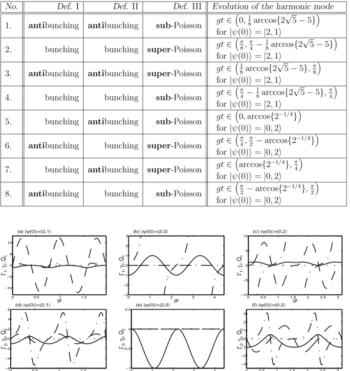
The evolution of the parameters Γ_i(t), γ_i(t) and Q_i(t) is given in Fig. 1(a) for the fundamental mode and in Fig. 1(d) for the harmonic mode.

We conclude that Defs. I and II are equivalent for the solution (11), i.e. antibunching I occurs whenever antibunching II occurs. However, Defs. I (or II) and III differ: sub-Poisson statistics of the fundamental mode can be accompanied by both bunching and antibunching (I or II). For the second mode all possible variations occur: (i) sub-Poisson statistics together with antibunching; (ii) sub-Poisson statistics together with bunching; (iii) super-Poisson statistics together with bunching; and (iv) super-Poisson statistics together with antibunching. The differences between sub-Poisson statistics and antibunching in SHG are only another example of the well-known facts (e.g., Refs. [7]–[9]).

Exact solution for |ψ(0)i = |2, 0i

The simplest nontrivial solution is for initial Fock fields |n₁, n₂i = |2, 0i; it takes the form

|ψ(t)i = cos x|2, 0i − i sin x|0, 1i, (16) where x =√

2gt. The mean photon numbers evolve as

hn1(t)i = 2 cos²x, hn2(t)i = sin²x. (17) We observe that both modes are unbunched according to Def. I, since Γ₁(t) = Γ₂(t) = 0. Applying Def. II, we find that the harmonic mode is also unbunched [γ₂(t) = 0]; however, the fundamental mode can be bunched, un- or antibunched since

γ₁(t) =√

2g sec²x tan x. (18)

According to Def. III, the fundamental mode can be sub-, super- or Poisson, but the harmonic mode cannot be super-Poisson

Q₁(t) = − cos x, Q₂(t) = − sin²x ≤ 0. (19) The evolution of the parameters Γ_i(t), γ_i(t) and Q_i(t) is given in Figs. 1(b) and 1(e). Again, we observe discrepancies between the single-time (Def. III) and two-time (Defs. I–II) correlation

(5)

functions. But the essential conclusion is that the predictions of Defs. I and II may be different for nonstationary evolution (16). Here, unbunching I is accompanied by antibunching II and bunching II. This example can provide a test of the validity of Def. II. One can interpret this case as follows:

normalization of G⁽²⁾(t, t + τ ) by a τ -dependent factor [e.g., G⁽¹⁾(t + τ )] introduces some artificial (phantom) anticorrelations.

TABLE I. All possible predictions of photon antibunching according to Defs. I, II, and III.

No. Def. I Def. II Def. III Evolution of the harmonic mode 1. antibunching antibunching sub-Poisson gt ∈^³0,¹₈arccos{2√

5 − 5}^´ for |ψ(0)i = |2, 1i

2. bunching bunching super-Poisson gt ∈^³^π₈,^π₄ − ¹₈arccos{2√

5 − 5}^´ for |ψ(0)i = |2, 1i

3. antibunching antibunching super-Poisson gt ∈^³¹₈arccos{2√

5 − 5},^π₈^´ for |ψ(0)i = |2, 1i

4. bunching bunching sub-Poisson gt ∈^³^π₄ − ¹₈arccos{2√

5 − 5},^π₄^´ for |ψ(0)i = |2, 1i

5. bunching antibunching sub-Poisson gt ∈^³0, arccos{2^−1/4}^´ for |ψ(0)i = |0, 2i

6. antibunching bunching super-Poisson gt ∈^³^π₄,^π₂ − arccos{2^−1/4}^´ for |ψ(0)i = |0, 2i

7. bunching antibunching super-Poisson gt ∈^³arccos{2^−1/4},^π₄^´ for |ψ(0)i = |0, 2i

8. antibunching bunching sub-Poisson gt ∈^³^π₂ − arccos{2^−1/4},^π₂^´ for |ψ(0)i = |0, 2i

0 0.5 1 1.5

−10

−5 0 5 10

Γ1, γ1, Q1

gt

(a) |ψ(0)〉=|2,1〉

0 1 2 3 4

−3

−2

−1 0 1 2 3

Γ1, γ1, Q1

gt

(b) |ψ(0)〉=|2,0〉

0 0.5 1 1.5 2 2.5 3

−10

−5 0 5 10

Γ1, γ1, Q1

gt

(c) |ψ(0)〉=|0,2〉

0 0.5 1 1.5

−6

−4

−2 0 2 4 6

Γ2, γ2, Q2

gt

(d) |ψ(0)〉=|2,1〉

0 1 2 3 4

−1

−0.5 0 0.5

Γ2, γ2, Q2

gt

(e) |ψ(0)〉=|2,0〉

0 0.5 1 1.5 2 2.5 3

−3

−2

−1 0 1 2 3

Γ2, γ2, Q2

gt

(f) |ψ(0)〉=|0,2〉

FIG. 1. Evolution of the parameters: Qi (solid lines), Γi (dashed) and γi (dot-dashed) for initial

(6)

Fock states |n1, n2i = |2, 1i, |2, 0i, |0, 2i. The parameters in figs. (a), (b), (c) are given for the fundamental mode (i = 1), and those in figs. (d), (e), (f) are for the harmonic mode (i = 2).

Exact solution for |ψ(0)i = |0, 2i

For initial Fock fields |n₁, n₂i = |0, 2i, we find the solution

|ψ(t)i = −

√3

2 sin²y|4, 0i − i

2sin(2y)|2, 1i + 1

4[3 + cos(2y)] |0, 2i, (20) where y = 2gt. This process describes subharmonic generation. The mean photon numbers are

hn₁(t)i = 1

2[5 − cos(2y)] sin²y, hn₂(t)i = 1

16[21 + 12 cos(2y) − cos(4y)] . (21) We observe, according to Def. I, that the fundamental and harmonic modes can be antibunched, unbunched or bunched:

Γ₁(t) = 12g sin²y sin(2y), Γ₂(t) = −g

2[3 + cos(2y)] sin(2y), (22) and according to Def. II:

γ₁(t) = −16g [13 cos y − 6 cos(3y) + cos(5y)] [5 − cos(2y)]⁻³csc³y,

γ₂(t) = 256g [106 cos y + 21 cos(3y) + cos(5y)] [21 + 12 cos(2y) − cos(4y)]⁻³sin³y. (23) Also, by applying Def. III, we find that both modes can have sub-, super- or Poisson statistics

Q₁(t) = 1

4[39 − 24 cos(2y) + cos(4y)] cos²y [5 − cos(2y)]⁻¹, Q₂(t) = − 1

32[419 + 600 cos(2y) + 28 cos(4y) − 24 cos(6y) + cos(8y)]

× [21 + 12 cos(2y) − cos(4y)]⁻¹. (24)

The evolution of the parameters Γ_i(t), γ_i(t) and Q_i(t) is presented in Figs. 1(c), 1(f).

As above, the predictions of Defs. I–II and III are different, i.e., antibunching I–II differs from antibunching III. But what is most intriguing, the predictions of Defs. I and II both for the fundamental and harmonic modes are opposite: antibunching I occurs whenever bunching II occurs and vice verse.

Table I shows discrepancies between Defs. I–III. It is seen that all possible cases (variations) occur in the evolution of the harmonic mode, e.g., from two initial states |2, 1i and |0, 2i. In order to observe all 8 cases for the fundamental mode one should take into account, e.g., the initial states |2, 1i and |0, 3i.

3 Conclusions

Up to now, as far as we know, photon antibunching defined by two-time correlation functions has hitherto not been studied in the SHG model. Besides. an analytical analysis of the sub-Poisson statistics in SHG has been given in the short-time approximation only [12].

(7)

We have found the exact analytical evolution of the fundamental and harmonic modes for some initial Fock states and applied these solutions in the analysis of the antibunching of photons in both modes according to Defs. I, II and III. The discrepancies between the definitions are summarized in Table I.

A comparison of the two-time and single-time correlations was presented just for the completeness of our discussion. The most important result of this paper is the comparison between the definitions based on the unnormalized (Def. I) and normalized (Def. II) two-time correlation functions. Defs. I and II coincide for stationary fields. However, for nonstationary fields, these definitions of photon antibunching describe distinct effects.

Acknowledgments. We are indebted to J. Peˇrina, M. Kozierowski and A. Ekert for valuable discussions. A.M. would like to thank A. Ekert for his hospitality at Oxford University. This work was supported by the grants: No. 2 PO3B 73 13 of the Polish Research Committee (KBN), No.

VS96028 of the Czech Ministry of Education and No. 202/96/0421 of the Czech Grant Agency, as well as the Hewlett-Packard grant for the Quantum Computation and Cryptography Group.

References

[1] H. J. Kimble, M. Dagenais and L. Mandel, Phys. Rev. Lett. 39, 691 (1977); M. Dagenais and L.

Mandel, Phys. Rev. A18, 2217 (1978).

[2] R. Short and L. Mandel, Phys. Rev. Lett. 51, 384 (1983).

[3] L. Mandel and E. Wolf, Optical Coherence and Quantum Optics (Cambridge Univ. Press, 1995) p.

712.

[4] J. Peˇrina, Z. Hradil and B. Jurˇco, Quantum Optics and Fundamentals of Physics (Kluwer, Dortrecht, 1994) p. 161.

[5] M. C. Teich and B. E. A. Saleh, in: Progress in Optics, ed. E. Wolf (North-Holland, Amsterdam, 1988), vol. 26, p. 1.

[6] H. Paul, Rev. Mod. Phys. 54, 1061 (1982).

[7] X. T. Zhou and L. Mandel, Phys. Rev. A 41, 475 (1990).

[8] S. Singh, Opt. Commun. 44, 254 (1983).

[9] H. T. Dung, A. S. Shumovsky and N. N. Bogolubov Jr., Opt. Commun. 90, 322 (1992); E. I.

Aliskenderov, H. T. Dung and L. Knll, Phys. Rev. A 48, 1604 (1993).

[10] D. Walls and R. Barakat, Phys. Rev. A1, 446 (1970); R. Tana´s, Ts. Gantsog and R. Zawodny, Quant.

Opt. 3, 221 (1991); R. Tana´s and Ts. Gantsog, Quant. Opt. 4, 254 (1991).

[11] J. Bajer, T. Opatrn´y and J. Peˇrina, Quant. Opt. 6, 403 (1994).

[12] M. Kozierowski and R. Tana´s, Opt. Comm. 21, 229 (1977); S. Kielich, M. Kozierowski and R. Tana´s, in: Coherence and Quantum Optics IV, eds. L. Mandel and E. Wolf (Plenum, New York, 1978) p.

511; L. Mandel, Opt. Comm. 42, 437 (1982); J. Peˇrina, V. Peˇrinov and J. Koˇdousek, Opt. Comm.

49, 210 (1984).