Prof. Fernando Quevedo: The Search for the Fundamental Theory of the Universe | Zapytaj Fizyka

The Search for the

Fundamental Theory of the Universe

Fernando Quevedo (Cambridge/ICTP-Trieste) Warsaw, Poland

Are we on the verge of a new revolution in science? De revolutionibus orbium

Greatest Recent Discoveries •  Fluctua2ons of Cosmic Microwave Background (1992) (Nobel Prize 2006) •  Dark Energy (1998) (Nobel Prize 2011) •  Higgs Discovery (2012) (Nobel Prize 2013) •  Gravita2onal waves (2016!) (Nobel Prize 2017)

Why are these discoveries important ?

Some Science History Highlights

(Understanding from Unifica2on )

Science Goals and Techniques

•  Explana'ons of physical phenomena

•  Asking well defined ques'ons

•  Making predic'ons, tes'ng predic'ons with

Science Tools

•  Human senses

•  Human brain:

1.  Curiousity

2.  Technology to go beyond our senses

Newton’s Unifica2on: Gravity

String Scenario n_s r f_{N L}

D3/anti D3 Inflation 0.92  n_s  0.93 r  10 5 f_{N L} ⌧ 1

DBI Inflation 0.93  n_s  0.96 10 x f_{N L}equil = 11 ± 69

Racetrack Inflation 0.95  n_s  0.96 r ⌧ 1 f_{N L} ⌧ 1

Wilson Line Inflation xxxx 0  r  0.12 0  f_{N L}  10

Kahler Moduli Inflation 0.96  n_s  0.967 < 10 12 0  f_{N L}  10

Fibre Inflation 0.965  n_s  0.97 0.007 r 0.0057 0  f_{N L}  25

Axion Monodromy 0.97  n_s  0.98 0.04  r  0.07 f_{N L}  1

D3/D7 Inflation 0.95  n_s  0.97 10 12  r  10 5 f_{N L}  1

Poly Instanton Inflation 0.95  n_s  0.97 10 12  r  10 5 f_{N L}  1

, x p ~ 2 (1) ~ = 1.05 ⇥ 10 34 _{Kg m}2 _/s

}

(2)

Complicated two-field inflationary model. Inflaton mostly an axion field. Hard to extract a simple, single field effective potential during inflation, since the single-field inflationary trajectory was found numerically. Also though it was the first successful case of closed string moduli inflation, the strong fine tuning makes them unattractive

theoretically at the moment. Small field inflation, almost gaussian and ns ⇠ 0.96.

2. Kahler Moduli

V_KM = A B 4/3 e a 4/3 (3)

with a a large constant a / V 2/3 with V ⇠ 105 ₁₀7 the large volume of the extra

dimensions. So despite the shape of the potential this is a small field inflationary

model with negligible tensor to scalar modes ratio. Inflationary scale 1013 GeV. The

relation between the spectral index and the number of e-folds is ns = 1 _N2

⇤ . Running

spectral index dn_s

d ln k =

4

N_⇤2 . The simplest models do not give non-gaussianities but

2

Gravity on earth

Gravity on space

Electricity + Magne2sm Unifica2on

Faraday and Maxwell

Electricity

Magnetism

Optics

String Scenario n_s r f_{N L}

D3/anti D3 Inflation 0.92  n_s  0.93 r  10 5 f_{N L} ⌧ 1

DBI Inflation 0.93  n_s  0.96 10 x f_{N L}equil = 11 ± 69

Racetrack Inflation 0.95  n_s  0.96 r ⌧ 1 f_{N L} ⌧ 1

Wilson Line Inflation xxxx 0  r  0.12 0  f_{N L}  10

Kahler Moduli Inflation 0.96  n_s  0.967 < 10 12 0  f_{N L}  10

Fibre Inflation 0.965  n_s  0.97 0.007 r 0.0057 0  f_{N L}  25

Axion Monodromy 0.97  n_s  0.98 0.04  r  0.07 f_{N L}  1

D3/D7 Inflation 0.95  n_s  0.97 10 12  r  10 5 f_{N L}  1

Poly Instanton Inflation 0.95  n_s  0.97 10 12  r  10 5 f_{N L}  1

, x p ~ 2 (1) ~ = 1.05 ⇥ 10 34 _{Kg m}2 _/s

}

(2)

Complicated two-field inflationary model. Inflaton mostly an axion field. Hard to extract a simple, single field effective potential during inflation, since the single-field inflationary trajectory was found numerically. Also though it was the first successful case of closed string moduli inflation, the strong fine tuning makes them unattractive

theoretically at the moment. Small field inflation, almost gaussian and ns ⇠ 0.96.

2. Kahler Moduli

V_KM = A B 4/3 e a 4/3 (3)

with a a large constant a / V 2/3 with V ⇠ 105 ₁₀7 the large volume of the extra

dimensions. So despite the shape of the potential this is a small field inflationary

model with negligible tensor to scalar modes ratio. Inflationary scale 1013 GeV. The

relation between the spectral index and the number of e-folds is ns = 1 _N2

⇤ . Running

spectral index dn_s

d ln k =

4

N_⇤2 . The simplest models do not give non-gaussianities but

2

Electromagnetism (Maxwell 1876)

Thermodynamics-Mechanics Unifica2on

(XVIII-XIX Century)

Heating slow particles Faster particles Increased temperature e.g. Temperature = average kine2c energy!!

Microscopic origin of macroscopic

quantities !

e.g. Entropy from number of states

Boltzmann constant:

Unifica2on of Space and Time

Special Rela2vity

Maximum (constant) speed: ‘speed of light’ c=3x108 m/s

Minkowski Spacetime

Unifica2on of Gravity and Space2me Geometry

Gravity and Geometry of Spacetime

Unifica2on of Par2cles and Waves

Quantum Fluctua2ons

String Scenario ns r fN L

D3/anti D3 Inflation 0.92 _{ ns  0.93} r _{ 10} 5 f_{N L ⌧ 1}

DBI Inflation 0.93 _{ ns  0.96} 10 x f_{N L}equil = 11 _{± 69}

Racetrack Inflation 0.95 _{ ns  0.96} r _{⌧ 1} f_{N L ⌧ 1}

Wilson Line Inflation xxxx 0 _{ r  0.12} 0 _{ f}N L  10

Kahler Moduli Inflation 0.96 _{ n}s  0.967 < 10 12 0  fN L  10 Fibre Inflation 0.965 _{ ns  0.97 0.007} r 0.0057 0 _{ fN L  25} Axion Monodromy 0.97 _{ ns  0.98} 0.04 _{ r  0.07} f_{N L  1}

D3/D7 Inflation 0.95 _{ ns  0.97} 10 12 _{ r  10} 5 f_{N L  1} Poly Instanton Inflation 0.95 _{ n}s  0.97 10 12  r  10 5 fN L  1

,

~ = 1.05 ⇥ 10 34 _{Kg m}2_/s 1. Racetrack

Complicated two-field inflationary model. Inflaton mostly an axion field. Hard to extract a simple, single field effective potential during inflation, since the single-field inflationary trajectory was found numerically. Also though it was the first successful case of closed string moduli inflation, the strong fine tuning makes them unattractive theoretically at the moment. Small field inflation, almost gaussian and ns _{⇠ 0.96.} 2. Kahler Moduli

V_KM = A B 4/3e a 4/3 (1)

with a a large constant a / V2/3 _{with V ⇠ 10}5 ₁₀7 _{the large volume of the extra} dimensions. So despite the shape of the potential this is a small field inflationary model with negligible tensor to scalar modes ratio. Inflationary scale 1013 GeV. The relation between the spectral index and the number of e-folds is ns = 1 _N2

⇤. Running

spectral index dns

d ln k =

4 N2

⇤ . The simplest models do not give non-gaussianities but

extensions of them can incorporate the curvaton mechanism for non-gaussianities with f_{N L ⇠ O(10).} 3. Fibre V_{f ibre} = V₀ 3 4e  (2) 2 String Scenario n_s r f_{N L} D3/anti D3 Inflation 0.92 _{ ns  0.93} r _{ 10} 5 f_{N L ⌧ 1}

DBI Inflation 0.93 _{ ns  0.96} 10 x f_{N L}equil = 11 _{± 69}

Racetrack Inflation 0.95 _{ ns  0.96} r _{⌧ 1} f_{N L ⌧ 1}

Wilson Line Inflation xxxx 0 _{ r  0.12} 0 _{ fN L  10}

Kahler Moduli Inflation 0.96 _{ n}s  0.967 < 10 12 0  fN L  10

Fibre Inflation 0.965 _{ ns  0.97 0.007} r 0.0057 0 _{ fN L  25}

Axion Monodromy 0.97 _{ ns  0.98} 0.04 _{ r  0.07} f_{N L  1}

D3/D7 Inflation 0.95 _{ n}s  0.97 10 12  r  10 5 fN L  1

Poly Instanton Inflation 0.95 _{ ns  0.97} 10 12 _{ r  10} 5 f_{N L  1}

,

x p ~

2 (1)

~ = 1.05 ⇥ 10 34 _{Kg m}2_/s

1. Racetrack

Complicated two-field inflationary model. Inflaton mostly an axion field. Hard to extract a simple, single field effective potential during inflation, since the single-field inflationary trajectory was found numerically. Also though it was the first successful case of closed string moduli inflation, the strong fine tuning makes them unattractive

theoretically at the moment. Small field inflation, almost gaussian and ns ⇠ 0.96.

2. Kahler Moduli

V_KM = A B 4/3e a 4/3 (2)

with a a large constant a / V2/3 with V ⇠ 105 ₁₀7 the large volume of the extra

dimensions. So despite the shape of the potential this is a small field inflationary

model with negligible tensor to scalar modes ratio. Inflationary scale 1013 GeV. The

relation between the spectral index and the number of e-folds is ns = 1 _N2_⇤ . Running

spectral index dns

d ln k =

4

N_⇤2 . The simplest models do not give non-gaussianities but

extensions of them can incorporate the curvaton mechanism for non-gaussianities with f_{N L ⇠ O(10).}

Unifica2on of Special Rela2vity and Quantum Mechanics

Dirac (+ Jordan Heisenberg, ..).

e.g. Quantum Electrodynamics (1948)

e.g. Electroweak Unifica2on

•  Higgs H spin=0

•  Graviton G spin=2 (Classical!?) 4 forces

3 Families + Higgs 3+1 Dimensions

Some Proper2es of the SM •  Arguably greatest theore2cal achievement in past 75 years. •  It is simple (not the simplest) •  It is ‘ugly’ (elegant principles but many free parameters) •  Not complete (baryogenesis, dark mafer, gravity)

Standard Model + Gravity

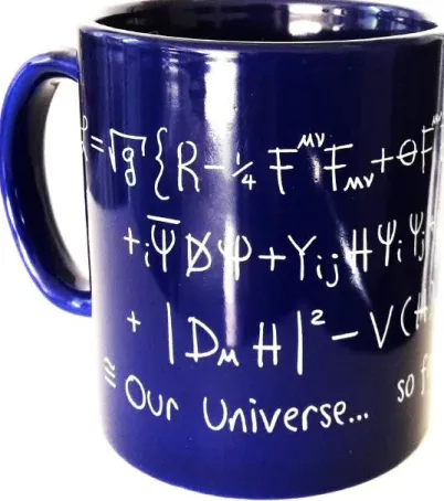
Figure 1: The standard model on a mug. The first row has the Einstein-Hilbert term for gravity ( = 2) and the kinetic and topological terms for the gauge fields ( = 1) describing the electromagnetic, weak and strong interactions. The second line has the kinetic energy for the matter fields: quarks and leptons = 1/2 as well as their (Yukawa) couplings to the Higgs field H ( = 0). The third line is the kinetic and potential energy for the Higgs field.

The robustness of the standard model is simply impressive. Other features to emphasise about the standard model (SM) are:

• The SM is an EFT. The non-gravitational part of the Lagrangian is renormalisable and therefore quantum mechanically complete (up to Landau poles). The inclusion of gravity makes it into an e↵ective field theory (EFT) which is well defined up to scales close to the Planck scale MP lanck =

p

~c/G ⇠ 1019 _{GeV. The fact that the non-gravitational part of}

the SM is renormalisable used to be regarded as a positive property. However, it is because of this property that we do not know at which scale the SM ceases to be valid and therefore we have less guidance of what lies beyond the SM. In this sense it could be possible that new physics may only manifest at or close to the Planck scale.

• The SM is simple but not the simplest. The structure of gauge fields and matter content of the SM is relatively simple (small rank simple gauge groups, matter in bi-fundamental representations). However, there are simpler gauge symmetries (such as just abelian U (1) symmetries or an SO(3) group) and matter content (only singlets, a single family, etc.) but they do not fit the experiments.

• Rich phase structure. The standard model is actually rich enough to illustrate most of the theoretically known phases of gauge theories: Coulomb phase (electromagnetism), Higgs

An Example: Our Universe!

Cosmic Microwave Background

Agree with Inflation! !!!

Open Ques2ons •  Why? (3+1 (dimensions, families, interac2ons); + some 20 parameters (masses, couplings)) •  Naturalness (hierarchy, cc, strong CP) •  ‘Technical’ (confinement,...) •  Cosmology (dark mafer, baryogenesis, density perturba2ons of CMB, origin/alterna2ves to infla2on,..., big-bang) •  Consistency (gravity)

Energy Distribution of the Universe

Bullet cluster (red x ray gas, blue dark matter, collision of two superclusters)

FUNDAMENTAL PROBLEM Quantum Gravity

= 1019 _GeV

String Theory?

String Theory

•  Particles ‘look like’ strings

•  Gravity is included

•  Can unify all particles and

interactions (Einstein’s dream)

•  Universe lives in 10 (11)

dimensions !!!

•  For our universe 10d = 4d+6d

(6d very small?)

•  Branes

•  New ‘fermionic’ dimensions

SUSY particles mass 1TeV solve hierarchy problem!!!

The Theory is Unique IIA IIB I Het 2 Het1 11D M

But many possible solutions or ‘vacua’ Each solution a different universe!!!

Landscape of Solutions

Each minimum universe with energy4 _{~ Λ!!!}

Multiverse

Anthropic explanation of dark energy?????

Many

General Progress •  Field is broad: Mathema2cs, cosmology, phenomenology, computer,... •  Aler the Higgs it is one of the main guides to Beyond Standard Model. •  Con2nuous ‘cumula2ve’ progress (infla2on, dark mafer candidates, etc.) •  The ‘Swampland’?

Landscape

Not consistent with quantum gravity Consistent with quantum gravity Swampland [Vafa’06] [Ooguri-Vafa’06]

Concrete Achievements •  Realis2c Model Building: Many quasi-realis2c models (local and global) but not fully realis2c yet. •  SUSY Breaking and Moduli Stabilisa2on: A handful of ‘scenarios’ (generically scalars much heavier than gauginos) •  Infla2on and pos2nfla2on cosmology: (Few scenarios with concrete predic2ons).

Holography !

(e.g.

Some Implica2ons of Holography

•  Proper defini2on of quantum gravity theory!

•  Black hole entropy/area! S_BH= (kc3/4Għ) A

Future? •  Experimentally driven? (LHC, axion search, post-Planck/experiments, Gravita2onal waves) (SUSY? Z’? non-gaussiani2es?, DR sefled? Tensor modes?) •  Accelerators: ILC, 100Km/100TeV hadron collider!? •  Evidence for String (GUT) scale physics?? (proton decay, cosmic strings, tensor modes, bubble collisions?...) •  Properly define the theory!!

String Models

•  Too many string models?

(>>10500₎

•  Or too ‘few’ models?

(Not fully Realistic model yet!!!)

Op2mis2c Perspec2ve •  Typical statement: “We do not understand well enough string theory to try to extract its physics implica'ons” •  Bold answer: “We may understand the theory beHer than we think (at low energies and weak couplings) using all foreseeable ingredients: geometry, branes, fluxes, perturba've, nonperturba've effects, etc.” ‘...our mistake is not that we take our theories too seriously, but that we do not take them seriously enough. It is always hard to realise that these numbers and equa'ons we play with at our desks have something to do with the real world.’ Steven Weinberg