Zrozumiały
Wszechświat
NOBEL 2019
Mikołaj Kopernik
1473 – 1543
1514
De Hypothesibus motuum coelestium… rozprawa
odnotowana w inwentarzu Macieja z Miechowa
1532
W zasadzie gotowy opis świata
1539-41
Wizyta Georga Joachima von Lauchena (Retyka),
który opracował streszczenie (wyd. 1540, Gdańsk) i zawiózł
rękopis do Norymbergi
1543
De revolutionibus orbium coelestium wychodzi drukiem
Ja w każdym razie mniemam, że ciężkość nie jest niczym innym,
jak tylko naturalną dążnością, którą boska opatrzność Stwórcy
wszechświata nadała częściom po to, żeby łączyły się w jedność
i całość, skupiając się razem w kształt kuli. A jest rzeczą godną
wiary, że taka dążność istnieje również w Słońcu, Księżycu
i innych świecących planetach, po to, by na skutek jej działania
trwały w tej krągłości, w jakiej nam się przedstawiają;
a niezależnie od tego w wieloraki sposób wykonują one swe ruchy
krążące.
Rys. B. Dwużnik, M. SzypułaGalileusz
1564 – 1642
(Galileo Galilei)
1589
stanowisko profesora matematyki na uniwersytecie w Pizie
1590
De Motu, doświadczenia ze spadkiem ciał
1592
przenosiny do Padwy
1609
obserwacje nieba własnoręcznie wykonaną lunetą
góry na Księżycu
gwiazdy Drogi Mlecznej
księżyce Jowisza
plamy na Słońcu, kształt Saturna, fazy Wenus
Sidereus Nuncius
12 III 1610
1623
Il Saggiatore – polemika z antagonistami
Filozofia zapisana jest w tej ogromnej księdze, którą
mamy stale otwartą przed naszymi oczami; myślę
o wszechświecie; jednakże nie można jej zrozumieć, jeśli
się wpierw nie nauczymy rozumieć języka i pojmować
znaki, jakimi została zapisana. Zapisana zaś została
w języku matematyki, a jej literami są trójkąty, koła
i inne figury geometryczne…
1610
nadworny matematyk Wielkiego Księcia Toskanii
ilustracje: WikipediaJames Peebles
ur. 1935
2019
Nagroda Nobla z fizyki
za odkrycia teoretyczne w zakresie kosmologii fizycznej
Zrozumiały
Wszechświat
= a(t)
0E = hc/
⇥ =
⇥
0a(t)
4Podstawowe prawo ewolucji Wszechświata
(równanie Friedmanna-Lemaitre’a)
Względne tempo rozszerzania
się Wszechświata
gęstość energii
wypełniającej Wszechświat
jest tym większe,
im większa jest
własności czasoprzestrzeni
materia/energia
R
µ⌫
1
2
Rg
µ⌫
=
8⇡G
c
4
T
µ⌫
E
= 3mc
2
V
= V
0
0
= E/V
E
= 3mc
2V
= a(t)
3V
0=
0a(t)
3pył (materia)
t
a t
“rozmiar”
⇥
Wszechświata
g¸esto´s´c
⇠
1
rozmiar
3
promieniowanie
g¸esto´s´c
⇠
1
rozmiar
4
D. Wilkinson
J. Peebles
R. Dicke
Bell Telephone Laboratories, ok. 1959
J. Pe eb le s, w yk ład n ob lo w sk iKoncepcja Wielkiego Wybuchu
w połowie lat 60. – pytania
•
Skąd we Wszechświecie wzięły się
poszczególne pierwiastki chemiczne?
•
Czy mikrofalowe promieniowanie tła ma jakąś
szczególną strukturę?
•
Z czego zbudowany jest Wszechświat?
•
Jak powstały galaktyki i gromady galaktyk?
Cząstki we Wszechświecie
••
^ +
^
••
!
_ +
••
_
••
zazdrość
••
_ +
_
••
!
^ +
••
^
••
Schadenfreude
••
_ +
^
••
!
^ +
••
_
••
zazdrość/ Schadenfreude
••
_
••
^
••
_
••
_
••
_
••
_
••
_
••
^
••
^
••
^
••
^
••
^
••
^
••
^
••
^
••
^
••
_
••
_
N = N
^
••+ N
_
••H = N
^
••N
_
••P (
⇥ nr 1
••
!
⇤) = (N
••
••
^
1)
P (
⇤ nr 1
••
!
⇥) = (N
••
••
_
1)
N
^••t
=
1
2
N
^••P (
••!
⇥) +
••1
2
N
_••P (
••⇥
!
••)
H
t
⇡
(N
2
••^
N
2
••_
) =
N H
t H••
^ +
^
••
!
_ +
••
_
••
••
_ +
^
••
!
^ +
••
_
••
zazdrość
••
_ +
_
••
!
^ +
••
^
••
Schadenfreude
zazdrość/ Schadenfreude
••
_
••
_
••
^
N = N
^
••+ N
_
••H = N
^
••N
_
••P (
⇥ nr 1
••
!
⇤) = (N
••
••
^
1)
N
^••t
=
1
2
N
^••P (
••!
⇥) +
••1
2
N
_••P (
••⇥
!
••)
H
t
=
↵N
2
••
^
=
↵
4
(N + H)
2
H
! N
Cząstki we Wszechświecie
••
^ +
^
••
!
_ +
••
_
••
••
_ +
_
••
!
^ +
••
^
••
••
_ +
^
••
!
^ +
••
_
••
zazdrość
Schadenfreude
zazdrość/ Schadenfreude
••
_
••
_
••
^
N = N
^
••+ N
_
••H = N
^
••N
_
•• t HUwzględnienie zmniejszającej się
w czasie gęstości i energii cząstek.
duża gęstość,
szybkie cząstki
wiele oddziaływań
mała gęstość,
powolne cząstki
brak oddziaływań
Cząstki we Wszechświecie
Nukleosynteza
powstanie pierwiastków
G. Gamov
F. Hoyle
Nukleosynteza
1 MeV
0.1 MeV
T
t
1s
2’
n
→
p
spada z 1/6 do 1/7
0.03 MeV
i wiele innych reakcji
…
neutrony trafiają do jąder
4He
bariera
kulombowska
Nukleosynteza
n + ⌫
$ p
+
+ e
p
+
+ n
! D +
2,2 MeV
p
+
+ n
! D +
2,2 MeV
Nukleosynteza
Peebles 1966
Mikrofalowe promieniowanie tła
13,6 eV
0,000235 eV 2,73 K
52
SCIENTIFIC AMERICAN FEBRUARY 2004BRYAN
CHRISTIE
DESIGN
GRAVITATIONAL MODULATION
INFLUENCE OF DARK MATTER
modulates the acoustic signals in
the CMB. After inflation, denser regions of dark matter that
have the same scale as the fundamental wave (represented as
troughs in this potential-energy diagram) pull in baryons and
photons by gravitational attraction. (The troughs are shown in
red because gravity also reduces the temperature of any
escaping photons.) By the time of recombination, about
380,000 years later, gravity and sonic motion have worked
together to raise the radiation temperature in the troughs
(blue) and lower the temperature at the peaks (red).
AT SMALLER SCALES,
gravity and acoustic pressure sometimes
end up at odds. Dark matter clumps corresponding to a
second-peak wave maximize radiation temperature in the troughs long
before recombination. After this midpoint, gas pressure pushes
baryons and photons out of the troughs (blue arrows) while
gravity tries to pull them back in (white arrows). This tug-of-war
decreases the temperature differences, which explains why the
second peak in the power spectrum is lower than the first.
Dark matter concentration Sonic motion Sonic motion Gravitational attraction Dark matter concentration Photon Baryon Gravitational attraction Photon BaryonFIRST PEAK
Gravity and sonic motion
work together
SECOND PEAK
Gravity counteracts
sonic motion
JUST AFT
ER INFLAT
ION
na podst. Hu & White, Sci. Am. 2004
silniejsza
grawitacja
przyciąganie
grawitacyjne
ruch
cząstek
POCZĄTEK
temperatu
ra
foton
barion
Korelacje temperatury na
określonych skalach kątowych
REKOMBIN
ACJA
zimniej
cieplej
MOO J1142+1527
1970ApJ...162..815P
2013
Planck
T = 2,73 K
T
T
⇠ 10
5
T
T
< 0,64
· 10
3
Bracewell & Conklin 1967
D. Shane
et al.
Groth & Peebles 1977
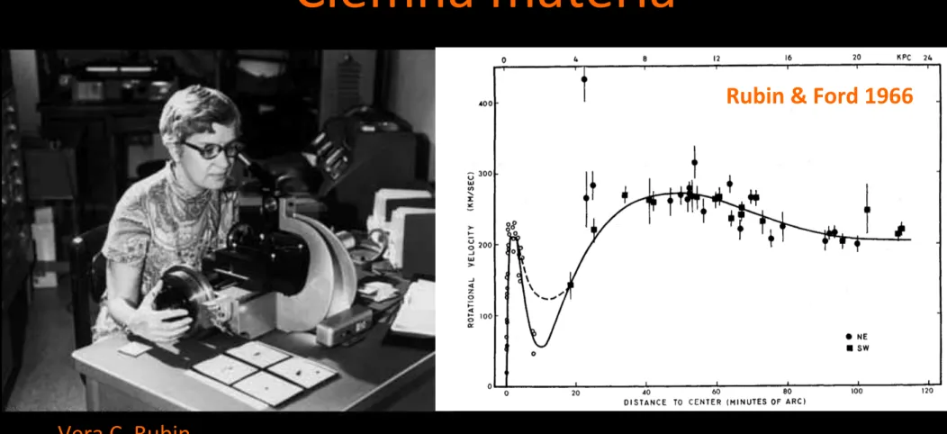
Ciemna materia
Ciemna materia
Vera C. Rubin
390 VERA C. RUBIN AND W. KENT FORD, JR.
24 kpc are 1.66 X ll11 Mo (low minimum) and 1.67 X 1111 Mo (higher minimum); those for the mass in the nucleus to = 1 kpc are 5.2 X 10⁹ Mo and 6.2 X 10⁹ Mo, respectively. When these values are increased 10 percent to compensate for the assump- tion of a flat disk (Brandt 1960), the total mass is 1.8 X 10¹¹ Mo out to 24 kpc. Also shown in Figure 10 are the variation in the mass surface density as a function of distance from the center, and the variation in the angular velocity, F/jR, as a function of R. Note that the solution with the high inner minimum has a positive mass density every- where. The solution with the low minimum has a negative surface density near 2? = 1 kpc. We take this to mean only that the density at this distance is vanishingly small for the low-minimum model.
Fig. 9.—Rotational velocities for OB associations in M31, as a function of distance from the center. Solid curve, adopted rotation curve based on the velocities shown in Fig. 4. For R < 12', curve is fifth- order polynomial; for R > 12', curve is fourth-order polynomial required to remain approximately flat near R — 120'. Dashed curve near i? = 10' is a second rotation curve with higher inner minimum. Various other rotation curves for the data in Figures 3 and 4 have been formed, all from least-squares solutions, with polynomials of third, fourth, or sixth order. In Figure 11 we show, superimposed, the fourteen rotation curves from the polynomial representa- tions. The various mass determinations from these rotation curves are listed in Table 4. Successive columns list the order of the polynomial, the resulting total mass, 1.1 times the mass, and the value of the maximum distance to which the mass has been deter- mined. The final columns list the depth of the inner minimum, and notes concerning the solutions.
It is apparent from the calculations that there is only a small spread in total mass out to i? = 24 kpc from all fourteen solutions. The shaded regions in Figure 12 indicate the range of masses which results from the fourteen rotation curves, as well as the range of surface densities. For the mass out to Æ = 24 kpc, a value of M = (1.68 ± 0.1) X ll11 Mg lies midway between all values. When this is increased 10 percent to compensate for the disk approximation, we obtain a mass M = (1.85 ± 0.1) X ll11 Mg out to
Æ = 24 kpc; the error is estimated from the total range in values. For the entire galaxy,
© American Astronomical Society • Provided by the NASA Astrophysics Data System
Ciemna materia
Ciemna materia
Vera C. Rubin
390 VERA C. RUBIN AND W. KENT FORD, JR.
24 kpc are 1.66 X ll11 Mo (low minimum) and 1.67 X 1111 Mo (higher minimum); those for the mass in the nucleus to = 1 kpc are 5.2 X 10⁹ Mo and 6.2 X 10⁹ Mo, respectively. When these values are increased 10 percent to compensate for the assump- tion of a flat disk (Brandt 1960), the total mass is 1.8 X 10¹¹ Mo out to 24 kpc. Also shown in Figure 10 are the variation in the mass surface density as a function of distance from the center, and the variation in the angular velocity, F/jR, as a function of R. Note that the solution with the high inner minimum has a positive mass density every- where. The solution with the low minimum has a negative surface density near 2? = 1 kpc. We take this to mean only that the density at this distance is vanishingly small for the low-minimum model.
Fig. 9.—Rotational velocities for OB associations in M31, as a function of distance from the center. Solid curve, adopted rotation curve based on the velocities shown in Fig. 4. For R < 12', curve is fifth- order polynomial; for R > 12', curve is fourth-order polynomial required to remain approximately flat near R — 120'. Dashed curve near i? = 10' is a second rotation curve with higher inner minimum. Various other rotation curves for the data in Figures 3 and 4 have been formed, all from least-squares solutions, with polynomials of third, fourth, or sixth order. In Figure 11 we show, superimposed, the fourteen rotation curves from the polynomial representa- tions. The various mass determinations from these rotation curves are listed in Table 4. Successive columns list the order of the polynomial, the resulting total mass, 1.1 times the mass, and the value of the maximum distance to which the mass has been deter- mined. The final columns list the depth of the inner minimum, and notes concerning the solutions.
It is apparent from the calculations that there is only a small spread in total mass out to i? = 24 kpc from all fourteen solutions. The shaded regions in Figure 12 indicate the range of masses which results from the fourteen rotation curves, as well as the range of surface densities. For the mass out to Æ = 24 kpc, a value of M = (1.68 ± 0.1) X ll11 Mg lies midway between all values. When this is increased 10 percent to compensate for the disk approximation, we obtain a mass M = (1.85 ± 0.1) X ll11 Mg out to
Æ = 24 kpc; the error is estimated from the total range in values. For the entire galaxy,
© American Astronomical Society • Provided by the NASA Astrophysics Data System
Rubin & Ford 1966
Figure 4: Two diagrams from 1974 that plot the relation between the mass and the radius of
galactic systems.
Left: the mass of spiral galaxies as a function of radius by Ostriker, Peebles
and Yahil (1974), as determined by various methods. Mass is in units of 10
12
M
J
.
Right:
the relation between mass and radius of Einasto, Kaasik and Saar (1974). The dots represent
the observed values obtained from pairs of galaxies, on the basis of data of Page (1970) and
Karachentsev (1966). The dashed line represents the mass function of known stellar populations;
the dotted line is the implied mass distribution of the ‘dark’ corona; the solid line is the total mass
distribution. Reproduced from ref. 15, AAS/IOP (left); and ref. 16, Macmillan Publishers Ltd
(right).
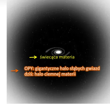
faint stars”. In this scenario, galaxies accounted for at least one-fifth of the critical
den-sity, ⌦
galaxies
0.2
. This value was sufficiently close to ⌦ = 1 to suggest agreement
with a closed universe, the authors implied. This somewhat generous extrapolation by
a factor of five is suggestive of the desirability of that cosmological scenario, which
was ”believed strongly by some”, the authors argued, ”for essentially nonexperimental
reasons”.
15
Motivated by similar arguments, an Estonian group at Tartu Obervatory,
consist-ing of Jaan Einasto, Ants Kaasik and Enn Saar, likewise concluded that the total mass
density of matter in galaxies is 20 percent of the critical cosmological density.
16
For
their influential paper (sent to Nature a few weeks before Ostriker et al. would
sub-mit their work—both articles came out months later), the Estonians used rotation curve
data of Roberts,
58
and masses of pairs of galaxies due to Thornton Page
94
and Igor
Karachentsev
38
, among others. From these data and their own, Einasto and his
co-workers constructed a diagram that plotted galaxy mass to radius similar to that of the
Princeton group, which showed the value of the extra mass a dark corona surrounding a
galaxy should have (see Fig. 4).
The Estonian group, just like its Princeton counterpart, was interdisciplinary in
interest and background: astronomers and theoretical physicists joined efforts to study
a problem that was now shared between galactic dynamics and cosmology. So, the
10
Ostriker, Peebles, Yahil 1974
świecąca materia
OPY: gigantyczne halo słąbych gwiazd
dziś: halo ciemnej materii
Ciemna materia
52
SCIENTIFIC AMERICAN
FEBRUARY 2004
BRYAN
CHRISTIE
DESIGN