Complex Analysis (Mathews + Howell)

Page iii

Complex Analysis for Mathematics and Engineering Third Edition

John H. Mathews

California State UniversityFullerton Russell W. Howell

Page iv World Headquarters

Jones and Bartlett Publishers 40 Tall Pine Drive

Sudbury, MA 01776 978-443-5000 info@jbpub.com www.jbpub.com

Jones and Bartlett Publishers Canada P.O. Box 19020

Toronto, ON M55 1X1 CANADA

Jones and Bartlett Publishers International Barb House, Barb Mews

London W6 7PA UK

Copyright ©1997 by Jones and Bartlett Publishers. © 1996 Times Mirror Higher Education Group. Inc.

All rights reserved. No part of this publication may be reproduced or transmitted in any form or by any means, electronic or mechanical, including photocopy, recording, or any information storage or retrieval system, without permission in writing from the publisher.

Library of Congress Catalog Number: 95-76589 ISBN 0-7637-0270-6

Printed in the United States of America 00 99 10 9 8 7 6 5 4 3

Page v

Contents

Preface ix

Chapter 1

Complex Numbers 1

1.1 The Origin of Complex Numbers 1 1.2 The Algebra of Complex Numbers 5 1.3 The Geometry of Complex Numbers 12 1.4 The Geometry of Complex Numbers, Continued 18 1.5 The Algebra of Complex Numbers, Revisited 24 1.6 The Topology of Complex Numbers 30 Chapter 2

Complex Functions 38

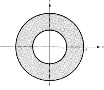
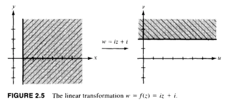
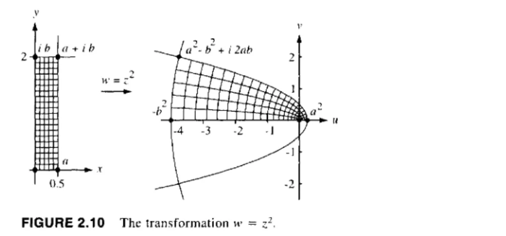
2.1 Functions of a Complex Variable 38 2.2 Transformations and Linear Mappings 41 2.3 The Mappings w = zn and w = z1/n 47

2.4 Limits and Continuity 53

2.5 Branches of Functions 60

2.6 The Reciprocal Transformation w = 1/z (Prerequisite for Section 9.2) 64 Chapter 3

Analytic and Harmonic Functions 71

3.1 Differentiable Functions 71

3.3 Analytic Functions and Harmonic Functions 84 Chapter 4

Sequences, Series, and Julia and Mandelbrot Sets 95 4.1 Definitions and Basic Theorems for Sequences and Series 95

4.2 Power Series Functions 109

Page vi Chapter 5

Elementary Functions 125

5.1 The Complex Exponential Function 125 5.2 Branches of the Complex Logarithm Function 132

5.3 Complex Exponents 138

5.4 Trigonometric and Hyperbolic Functions 143 5.5 Inverse Trigonometric and Hyperbolic Functions 152 Chapter 6

Complex Integration 157

6.1 Complex Integrals 157

6.2 Contours and Contour Integrals 160

6.3 The Cauchy-Goursat Theorem 175

6.4 The Fundamental Theorems of Integration 189 6.5 Integral Representations for Analytic Functions 195 6.6 The Theorems of Morera and Liouville and Some

Applications 201

Chapter 7

Taylor and Laurent Series 208

7.1 Uniform Convergence 208

7.2 Taylor Series Representations 214 7.3 Laurent Series Representations 223 7.4 Singularities, Zeros, and Poles 232

7.5 Applications of Taylor and Laurent Series 239 Chapter 8

Residue Theory 244

8.1 The Residue Theorem 244

8.2 Calculation of Residues 246

8.3 Trigonometric Integrals 252

8.4 Improper Integrals of Rational Functions 256 8.5 Improper Integrals Involving Trigonometric Functions 260

8.6 Indented Contour Integrals 264

8.7 Integrands with Branch Points 270 8.8 The Argument Principle and Rouché's Theorem 274 Chapter 9

Conformal Mapping 281

9.1 Basic Properties of Conformal Mappings 281

9.2 Bilinear Transformations 287

9.3 Mappings Involving Elementary Functions 294 9.4 Mapping by Trigonometric Functions 303

Page vii Chapter 10

Applications of Harmonic Functions 310

10.1 Preliminaries 310

10.2 Invariance of Laplace's Equation and the Dirichlet Problem 312 10.3 Poisson's Integral Formula for the Upper Half Plane 323 10.4 Two-Dimensional Mathematical Models 327

10.5 Steady State Temperatures 329

10.6 Two-Dimensional Electrostatics 342 10.7 Two-Dimensional Fluid Flow 349

10.8 The Joukowski Airfoil 360

10.9 The Schwarz-Christoffel Transformation 369

10.10 Image of a Fluid Flow 380

10.11 Sources and Sinks 384

Chapter 11

Fourier Series and the Laplace Transform 397

11.1 Fourier Series 397

11.2 The Dirichlet Problem for the Unit Disk 406 11.3 Vibrations in Mechanical Systems 412

11.4 The Fourier Transform 418

11.5 The Laplace Transform 422

11.7 Shifting Theorems and the Step Function 433 11.8 Multiplication and Division by t 438 11.9 Inverting the Laplace Transform 441

11.10 Convolution 448

Appendix A

Undergraduate Student Research Projects 456

Bibliography 458

Answers to Selected Problems 466

Preface

Approach This text is intended for undergraduate students in mathematics,

physics, and engineering. We have attempted to strike a balance between the pure and applied aspects of complex analysis and to present concepts in a clear writing style that is understandable to students at the junior or senior undergraduate level. A wealth of exercises that vary in both difficulty and substance gives the text flex-ibility. Sufficient applications are included to illustrate how complex analysis is used in science and engineering. The use of computer graphics gives insight for understanding that complex analysis is a computational tool of practical value. The exercise sets offer a wide variety of choices for computational skills, theoretical understanding, and applications that have been class tested for two editions of the text. Student research projects are suggested throughout the text and citations are made to the bibliography of books and journal articles.

The purpose of the first six chapters is to lay the foundations for the study of complex analysis and develop the topics of analytic and harmonic functions, the elementary functions, and contour integration. If the goal is to study series and the residue calculus and applications, then Chapters 7 and 8 can be covered. If con-formal mapping and applications of harmonic functions are desired, then Chapters 9 and 10 can be studied after Chapter 6. A new Chapter 11 on Fourier and Laplace transforms has been added for courses that emphasize more applications.

Proofs are kept at an elementary level and are presented in a self-contained manner that is understandable for students having a sophomore calculus back-ground. For example, Green's theorem is included and it is used to prove the Cauchy-Goursat theorem. The proof by Goursat is included. The development of series is aimed at practical applications.

Features Conformal mapping is presented in a visual and geometric manner so

that compositions and images of curves and regions can be understood. Boundary value problems for harmonic functions are first solved in the upper half-plane so that conformal mapping by elementary functions can be used to find solutions in other domains. The Schwarz-Christoffel formula is carefully developed and appli-cations are given. Two-dimensional mathematical models are used for appliappli-cations in the area of ideal fluid flow, steady state temperatures and electrostatics. Computer drawn figures accurately portray streamlines, isothermals, and equipotential curves. New for this third edition is a historical introduction of the origin of complex numbers in Chapter 1. An early introduction to sequences and series appears in Chapter 4 and facilitates the definition of the exponential function via series. A new section on the Julia and Mandelbrot sets shows how complex analysis is connected

x Preface

to contemporary topics in mathematics. Many sections have been revised including branches of functions, the elementary functions, and Taylor and Laurent series. New material includes a section on the Joukowski airfoil and an additional chapter on Fourier series and Laplace transforms. Modern computer-generated illustrations have been introduced in the third edition including: Riemann surfaces, contour and surface graphics for harmonic functions, the Dirichlet problem, streamlines in-volving harmonic and analytic functions, and conformal mapping.

Acknowledgments We would like to express our gratitude to all the people whose

efforts contributed to the development and preparation of the first edition of this book. We want to thank those students who used a preliminary copy of the manu-script. Robert A. Calabretta, California State University-Fullerton, proofread the manuscript. Charles L. Belna, Syracuse University, offered many useful suggestions and changes. Edward G. Thurber, Biola University, used the manuscript in his course and offered encouragement. We also want to thank Richard A. Alo, Lamar University; Arlo Davis, Indiana University of Pennsylvania; Holland Filgo, North-eastern University; Donald Hadwin, University of New Hampshire; E. Robert Heal, Utah State University; Melvin J. Jacobsen, Rensselaer Polytechnic Institute; Charles P. Luehr, University of Florida; John Trienz, United States Naval Academy; William Trench, Drexel University; and Carroll O. Wilde, Naval Postgraduate School, for their helpful reviews and suggestions. And we would like to express our gratitude to all the people whose efforts contributed to the second edition of the book. Our colleagues Vuryl Klassen, Gerald Marley, and Harris Schultz at California State University-Fullerton; Arlo Davis, Indiana University of Pennsylvania; R. E. Wil-liamson, Dartmouth College; Calvin Wilcox, University of Utah; Robert D. Brown, University of Kansas; Geoffrey Price, U.S. Naval Academy; and Elgin H. Johnston, Iowa State University.

For this third edition we thank our colleague C. Ray Rosentrater of Westmont College for class testing the material and for making many valuable suggestions. In addition, we thank T. E. Duncan, University of Kansas; Stuart Goldenberg, Cali-fornia Polytechnic State University-San Luis Obispo; Michael Stob, Calvin College; and Vencil Skarda, Brigham Young University, for reviewing the manuscript.

In production matters we wish to express our appreciation to our copy editor Pat Steele and to the people at Wm. C. Brown Publishers, especially Mr. Daryl Bruflodt, Developmental Editor, Mathematics and Gene Collins, Senior Production Editor, for their assistance.

The use of computer software for symbolic computations and drawing graphs is acknowledged by the authors. Many of the graphs in the text have been drawn with the F(Z)™, MATLAB®, Maple™, and Mathematica™ software. We wish to thank the people at Art Matrix for the color plate pictures in Chapter 4. The authors have developed supplementary materials available for both IBM and Macintosh

Preface xi computers, involving the abovementioned software products. Instructors who use the text may contact the authors directly for information regarding the availability of the F(Z)™, MATLAB®, Maple™, and Mathematica™ supplements. The authors appreciate suggestions and comments for improvements and changes to the text. Correspondence can be made directly to the authors via surface or e-mail.

John Mathews Dept. of Mathematics

California State University-Fullerton Fullerton, CA 92634

mathews@fullerton.edu Russell Howell

Dept. of Mathematics and Computer Science Westmont College

Santa Barbara, CA 93108 howell @ westmont.edu

1

Complex

Numbers

1.1 The Origin of Complex Numbers

Complex analysis can roughly be thought of as that subject which applies the ideas of calculus to imaginary numbers. But what exactly are imaginary numbers? Usu-ally, students learn about them in high school with introductory remarks from their teachers along the following lines: "We can't take the square root of a negative number. But, let's pretend we can—and since these numbers are really imaginary, it will be convenient notationally to set i = v ^ ^ " Rules are then learned for doing arithmetic with these numbers. The rules make sense. If i = >/--T, it stands to reason that i2 = -1. On the other hand, it is not uncommon for students to wonder all along whether they are really doing magic rather than mathematics.

If you ever felt that way, congratulate yourself! You're in the company of some of the great mathematicians from the sixteenth through the nineteenth centu-ries. They too were perplexed with the notion of roots of negative numbers. The purpose of this section is to highlight some of the episodes in what turns out to be a very colorful history of how imaginary numbers were introduced, investigated, avoided, mocked, and, eventually, accepted by the mathematical community. We intend to show you that, contrary to popular belief, there is really nothing imaginary about "imaginary numbers" at all. In a metaphysical sense, they are just as real as are "real numbers."

Our story begins in 1545. In that year the Italian mathematician Girolamo Cardano published Ars Magna (The Great Art), ZL 40-chapter masterpiece in which he gave for the first time an algebraic solution to the general cubic equation

x3, + ax2 + bx + c = 0.

His technique involved transforming this equation into what is called a depressed

cubic. This is a cubic equation without the x2 term, so that it can be written as

x3 + bx + c = 0.

Cardano knew how to handle this type of equation. Its solution had been communicated to him by Niccolo Fontana (who, unfortunately, came to be known as Tartaglia—the stammerer—because of a speaking disorder). The solution was

2 Chapter 1 Complex Numbers

also independently discovered some 30 years earlier by Scipione del Ferro of Bo-logna. Ferro and Tartaglia showed that one of the solutions to the depressed cubic is

K J V 2 V4 27 \ 2 V 4 27

This value for x could then be used to factor the depressed cubic into a linear term and a quadratic term, the latter of which could be solved with the quadratic formula. So, by using Tartaglia's work, and a clever transformation technique, Cardano was able to crack what had seemed to be the impossible task of solving the general cubic equation.

It turns out that this development eventually gave a great impetus toward the acceptance of imaginary numbers. Roots of negative numbers, of course, had come up earlier in the simplest of quadratic equations such as x2: + 1 = 0. The solutions we know today as x = ±7~^~» however, were easy for mathematicians to ignore. In Cardano's time, negative numbers were still being treated with some suspicion, so all the more was the idea of taking square roots of them. Cardano himself, al-though making some attempts to deal with this notion, at one point said that quan-tities such as ^--1 were "as subtle as they are useless." Many other mathematicians also had this view. However, in his 1572 treatise Algebra, Rafael Bombeli showed that roots of negative numbers have great utility indeed. Consider the simple de-pressed cubic equation JC3 — 15JC — 4 = 0. Letting b = —15 and c = —4 in the

"Ferro-Tartaglia" formula (1), we can see that one of the solutions for x is

Bombeli suspected that the two parts of x in the preceding equation could be put in the form u + v 7 ~ l and — u + vJ—\ for some numbers u and v. Indeed, using the well-known identity {a + b)3 = a3 + 3a2b + 3ab2 + b39 and blindly pretending that roots of negative numbers obey the standard rules of algebra, we can see that

(2) (2 + y ^ T )3 = 23 + 3(22) v ^ T + 3(2)0

= 8 + 1 2 7 ^ 1 6 -= 2 + l l v ^ T = 2 + 7 - 1 2 1 .

Bombeli reasoned that if (2 + 7 - T )3 = 2 + 7 - 1 2 1 , it must be that 2 + 7 ~ T

= Ijl + 7 - 7 2 L Likewise, he showed - 2 + 7 ^ 1 = ^ - 2 + 7 - 1 2 1 . But then we clearly have

(3) Ul +

J^UA - ^-2 + T

! ^

= (2 +

T

! )

- (-2 +

T^T)

= 4,

1.1 The Origin of Complex Numbers 3

territory of ''imaginary numbers." Thus, whatever else one might say about these numbers (which, today, we call complex numbers), their utility could no longer be ignored.

But even this breakthrough did not authenticate complex numbers. After all, a real number could be represented geometrically on the number line. What possible representation could these new numbers have? In 1673 John Wallis made a stab at a geometric picture of complex numbers that comes close to what we use today. He was interested at the time in representing solutions to general quadratic equations, which we shall write as x2 + 2bx + c2 = 0 so as to make the following discussion more tractable. Using the quadratic formula, the preceding equation has solutions

x — -b- Jb2 and

=

-fc

+

JW

Wallis imagined these solutions as displacements to the left and right from the point —b. He saw each displacement, whose value was Jb2 — c2, as the length

of the sides of the right triangles shown in Figure 1.1.

P] (-/7,0) P2 (0,0)

FIGURE 1.1 Wallis' representation of real roots of quadratics.

The points Pi and P2 in this figure are the representations of the solutions to

our equation. This is clearly correct if b2 — c2 > 0, but how should we picture Pi

and P2 in the case when negative roots arise—i.e., when b2 — c2 < 0? Wallis reasoned that if this happened, b would be less than c, so the lines of length b in Figure 1.1 would no longer be able to reach all the way to the x axis. Instead, they would stop somewhere above it, as Figure 1.2 shows. Wallis argued that P\ and P2

should represent the geometric locations of the solutions x = — b — Jb2 — c2 and

x = — b + Jb2 — c2 in the case when b2 — c2 < 0. He evidently thought that since

b is shorter than c, it could no longer be the hypotenuse of the right triangle as it

had been earlier. The side of length c would now have to take that role.

(-b, 0) (0, 0)

4 Chapter 1 Complex Numbers

Wallis' method has the undesirable consequence that — J— 1 is represented by the same point as is J^X. Nevertheless, with this interpretation, the stage was set for thinking of complex numbers as ''points in the plane." By 1800, the great Swiss mathematician Leonard Euler (pronounced "oiler") adopted this view con-cerning the n solutions to the equation xn — 1 = 0. We shall learn shortly that these solutions can be expressed as cos 6 + J^-\ sin 6 for various values of 6; Euler thought of them as being located at the vertices of a regular polygon in the plane. Euler was also the first to use the symbol i for V ^ T . Today, this notation is still the most popular, although some electrical engineers prefer the symbol j instead so that i can be used to represent current.

Perhaps the most influential figure in helping to bring about the acceptance of complex numbers was the brilliant German mathematician Karl Friedrich Gauss, who reinforced the utility of these numbers by using them in his several proofs of the fundamental theorem of algebra (see Chapter 6). In an 1831 paper, he produced a clear geometric representation of x 4- iy by identifying it with the point (x, y) in the coordinate plane. He also described how these numbers could be added and multiplied.

It should be noted that 1831 was not the year that saw complex numbers transformed into legitimacy. In that same year the prolific logician Augustus De Morgan commented in his book On the Study and Difficulties of Mathematics, "We have shown the symbol J^a to be void of meaning, or rather self-contradictory and absurd. Nevertheless, by means of such symbols, a part of algebra is established which is of great utility." To be sure, De Morgan had raised some possible logical problems with the idea of complex numbers. On the other hand, there were sufficient answers to these problems floating around at the time. Even if De Morgan was unaware of Gauss' paper when he wrote his book, others had done work similar to that of Gauss as early as 1806, and the preceding quote illustrates that "raw logic" by itself is often insufficient to sway the entire mathematical community to adopt new ideas. Certainly, logic was a necessary ingredient in the acceptance of complex numbers, but so too was the adoption of this logic by Gauss, Euler, and others of "sufficient clout." As more and more mathematicians came to agree with this new theory, it became socially more and more difficult to raise objections to it. By the end of the nineteenth century, complex numbers were firmly entrenched. Thus, as it is with any new mathematical or scientific theory, the acceptance of complex numbers came through a mixture of sociocultural interactions.

But what is the theory that Gauss and so many others helped produce, and how do we now think of complex numbers? This is the topic of the next few sections.

EXERCISES FOR SECTION 1.1

1. Give an argument to show that - 2 + y ^ T = ^/-2 + ,/-121.

2. Explain why cubic equations, rather than quadratic equations, played the pivotal role in helping to obtain the acceptance of complex numbers.

3. Find all solutions to 27x3 - 9x — 2 = 0. Hint: Get an equivalent monic polynomial,

1.2 The Algebra of Complex Numbers 5

4. By inspection, one can see that a solution to x3 - 6x + 4 = 0 is x = 2. To get an idea

of the difficulties Bombeli had in establishing identities (2) and (3) in the text, try to show how the solution x = 2 arises when using formula (1).

5. Explain why Wallis' view of complex numbers results in - ^ ^ 1 being represented by

the same point as is y/--\. ' 6. Is it possible to modify slightly Wallis' picture of complex numbers so that it ii

con-sistent with the representation we use today? To assist in your investigation of this question, we recommend the following article: Norton, Alec, and Lotto, Benjamin, "Complex Roots Made Visible," The College Mathematics Journal, Vol. 15 (3), June 1984, pp. 248-249.

7. Write a report on the history of complex analysis. Resources include bibliographical items 87, 105, and 179.

1.2 The Algebra of Complex Numbers

We have seen that complex numbers came to be viewed as ordered pairs of real numbers. That is, a complex number z is defined to be

(1) z = (x,y),

where x and y are both real numbers.

The reason we say ordered pair is because we are thinking of a point in the plane. The point (2, 3), for example, is not the same as (3, 2). The order in which we write x and v in equation (1) makes a difference. Clearly, then, two complex numbers are equal if and only if their x coordinates are equal and their y coordinates are equal. In other words,

(x, y) = (w, v) iff x = u and y = v. (Throughout this text, iff means if and only if.)

If we are to have a meaningful number system, there needs to be a method for combining these ordered pairs. We need to define algebraic operations in a consis-tent way so that the sum, difference, product, and quotient of any two ordered pairs will again be an ordered pair. The key to defining how these numbers should be manipulated is to follow Gauss' lead and equate (x, y) with x + iy. Then, by letting

Z\ = (xi,y\) and z2 = (x2, y2) be arbitrary complex numbers, we see that z\ + zi = (xuy{) + (x2,y2)

= (*\ + iy\) + to + iyi) = (*\ + *2) + Ky\ + yi) = (*\ + *2. y\ +

yi)-Thus, the following should certainly make sense:

Definition for addition

(2) Z\ + z2 = (xuyi) + (x2,y2)

yi)-6 Chapter 1 Complex Numbers

Definition for subtraction

(3) z\ - z2 = (xuyi) ~ (x2,y2)

= (x{ - x2, y\ - y2).

E X A M P L E 1.1 If Z\ = (3, 7) and z2 = (5, - 6 ) , then

z\ + zi - (3, 7) + (5, - 6 ) = (8, 1) and zx - 2 2 = ( 3 , 7 ) - ( 5 , - 6 ) = ( - 2 , 1 3 ) .

At this point, it is tempting to define the product z\Zi as Z\Zt = {xxx2, yiyi)- It turns out, however, that this is not a good definition, and you will be asked in the problem set for this section to explain why. How, then, should products be defined? Again, if we equate (JC, y) with x + iy and assume, for the moment, that i - V-l makes sense (so that i2 = -1), we have

z\Zi = (xu yi)(x2, y2)

= (x[ + iy\)(x2 + iy2)

= xxx2 + ixxy2 + ixzyi + i2y\y2 = x{x2 - y{y2 + i(xiy2 + x2yx) = (x\x2 - yiy2, xxy2 + x2yx).

Thus, it appears we are forced into the following definition.

Definition for multiplication

(4) z\z2 = (xu yx)(x2, y2)

= (x{x2 - ^,y2, xiy2 + x2y{).

E X A M P L E 1.2 If Z\ = (3, 7) and z2 = (5, - 6 ) , then

ziz2 = (3, 7)(5, - 6 ) = (15 + 42, - 1 8 + 35) = (57, 17).

Note that this is the same answer that would have been obtained if we had used the notation z\ — 3 + li and z2 = 5 — 6/. For then

zizi = (3, 7)(5, - 6 ) = (3 + 7/)(5 - 6/) = 15 - 18/ + 35/ - 42/2 = 15 - 42(-1) + ( - 1 8 + 35)/ = 57 + 17/ = (57, 17).

1.2 The Algebra of Complex Numbers 7

Of course, it makes sense that the answer came out as we expected, since we used the notation x + iy as motivation for our definition in the first place.

To motivate our definition for division, we will proceed along the same lines as we did for multiplication, assuming z2 ^ 0.

Z]_ _ ( * i , ; y i )

zi (x2, y2)

= (x\ + iyi)

(x2 + iy2)'

At this point we need to figure out a way to be able to write the preceding quantity in the form x + iy. To do this, we use a standard trick and multiply the numerator and denominator by x2 — iy2. This gives

z± = (x\ + iyi) (x2 - iy2)

z2 (x2 + iy2) (x2 - iy2)

_ *\*2 + y\yi m-xiy2 + *2y\

x\ + y\ xj + y\ x{x2 + yxy2 -xxy2 + x2y\

x\ + y\ x\ + y\

Thus, we finally arrive at a rather odd definition.

Definition for division Z\ (xuyx) (5) z2 (x2, y2) {xxx2 + yxy2 -x\y2 + *2y\ , f , n E X A M P L E 1.3 If Z\ = (3, 7) and z2 = (5, - 6 ) , then z\ (3,7) / 1 5 - 4 2 18 + 3 5 \ / - 2 7 53 z2 (5, - 6 ) \25 + 36 25 + 36/ \ 61 61

8 Chapter 1 Complex Numbers

As we saw with the example for multiplication, we will also get this answer if we use the notation x + iy:

Zx _ (3, 7) z2 (5, - 6 ) _ 3 + li ~ 5 - 6/ _ 3 + li 5 + 6/ ~~ 5 - 6/ 5 + 6/ _ 15 + 18/ + 35/ + 42/2 ~ 25 + 30/ - 30/ - 36/2 _ 15 - 42 + (18 + 35)/ 25 + 36 - 2 7 53 = + —/ 61 61

_ (zH *l\

The technique most mathematicians would use to perform operations on com-plex numbers is to appeal to the notation x + iy and perform the algebraic manip-ulations, as we did here, rather than to apply the complicated looking definitions we gave for those operations on ordered pairs. This is a valid procedure since the

x + iy notation was used as a guide to see how we should define the operations in

the first place. It is important to remember, however, that the x 4- iy notation is nothing more than a convenient bookkeeping device for keeping track of how to manipulate ordered pairs. It is the ordered pair algebraic definitions that really form the foundation on which our complex number system is based. In fact, if you were to program a computer to do arithmetic on complex numbers, your program would perform calculations on ordered pairs, using exactly the definitions that we gave.

It turns out that our algebraic definitions give complex numbers all the prop-erties we normally ascribe to the real number system. Taken together, they describe what algebraists call afield. In formal terms, a field is a set (in this case, the complex numbers) together with two binary operations (in this case, addition and multipli-cation) with the following properties:

(PI) Commutative law for addition: z\ + Zi = Zi + Z\.

(P2) Associative law for addition: z\ + fe + Zs) — (zi + Zi) + Z3.

(P3) Additive identity: There is a complex number co such that z + co = z for all

complex numbers z- The number a> is obviously the ordered pair (0, 0).

(P4) Additive inverses: Given any complex number z, there is a complex

number r\ (depending on z) with the property that z + r| = (0, 0). Obviously, if z = (x, y) = x + iy, the number r| will be

1.2 The Algebra of Complex Numbers 9 (PS) Commutative law for multiplication: z\z2 = z2Z\.

(P6) Associative law for multiplication: zAziz?) = (Z]Z2)zi.

(P7) Multiplicative identity: There is a complex number £ such that z£> = z for

all complex numbers z. It turns out that (1, 0) is the complex number £ with this property. You will be asked to verify this in the problem set for this section.

(P8) Multiplicative inverses: Given any complex number z other than the

number (0, 0), there is a complex number (depending on z) which we shall denote by z~l with the property that zz~l = (1,0). Given our definition for division, it seems reasonable that the number z~l would be z~] = —!— .

z You will be asked to confirm this in the problem set for this section.

(P9) The distributive law: z\{z2 + Z3) = Z\Z2 + Z\Z3.

None of these properties is difficult to prove. Most of the proofs make use of corresponding facts in the real number system. To illustrate this, we give a proof of property PI.

Proof of the commutative law for addition Let z\ = (xu yO and

z2 ~ (*2> yi) he arbitrary complex numbers. Then,

z\ + z2 = (*i,yi) + (*2, y2)

= (X, + X2i Vi + V2) = (x2 + xl9y2 + ^1)

= (x29y2) + 0cuy\) = Z2+ Z\.

The real number system can actually be thought of as a subset of our complex number system. To see why this is the case, let us agree that since any complex number of the form (t, 0) is on the x axis, we can identify it with the real number t. With this correspondence, it is easy to verify that the definitions we gave for ad-dition, subtraction, multiplication, and division of complex numbers are consistent with the corresponding operations on real numbers. For example, if x\ and x2 are real numbers, then

X\X2 = (jti, 0)(x2, 0) (by our agreed correspondence)

= (x\X2 — 0, 0 + 0) (by definition of multiplication of complex numbers) = (x\X2, 0) (confirming the consistency of our correspondence). It is now time to show specifically how the symbol i relates to the quantity y1 7! . Note that

(0, 1)2 = (0, 1)(0, 1)

= (0 — 1,0 + 0) (by definition of multiplication of complex numbers) = ( - 1 , 0 )

= — 1 (by our agreed correspondence).

(by definition of addition of complex numbers) (by the commutative law for real numbers) (by definition of addition of complex numbers)

10 Chapter 1 Complex Numbers

If we use the symbol i for the point (0, 1), the preceding gives i2 = (0, 1)2 = - 1 ,

which means i = (0, 1) = J~—\. So, the next time you are having a discussion with your friends, and they scoff when you claim that J^-\ is not imaginary, calmly put your pencil on the point (0, 1) of the coordinate plane and ask them if there is anything imaginary about it. When they agree there isn't, you can tell them that this point, in fact, represents the mysterious ^f-\ in the same way that (1,0) represents 1.

We can also see more clearly now how the notation x + iy equates to (x, y). Using the preceding conventions, we have

/ m i /n i\/ r^ (by our previously discussed conventions, * + ,? = (*, 0) + (0, i)(y,o) ^= p ( J C > 0 X e t y c )

= (x, 0) + (0, y) (by definition of multiplication of complex numbers) = (x, y) (by definition of addition of complex numbers). Thus, we may move freely between the notations x + iy and (x, y), depending on which is more convenient for the context in which we are working.

We close this section by discussing three standard operations on complex numbers. Suppose z = U, y) = x + iy is a complex number. Then:

(i) The real part of z, denoted by Re(z), is the real number x. (ii) The imaginary part of z, denoted by Im(z), is the real number y.

(iii) The conjugate of z, denoted by z, is the complex number (x, —y) = x — iy.

EXAMPLE 1.4

EXAMPLE 1.5

EXAMPLE 1.6

The following are some important facts relating to these operations that you will be asked to verify in the exercises:

(6)

Re(

)

=

i ± i .

z-z

1.2 The Algebra of Complex Numbers 11

(10) zizi = u zi-(11) ! = z.

(12) Re(fe) - - I m ( z ) . (13) Im(iz) = Re(z).

Because of what it erroneously connotes, it is a shame that the term imaginary is used in definition (ii). Gauss, who was successful in getting mathematicians to adopt the phrase complex number rather than imaginary number, also suggested that we use lateral part of z in place of imaginary part of z. Unfortunately, this sugges-tion never caught on, and it appears we are stuck with the words history has handed down to us.

EXERCISES FOR SECTION 1.2

1. Perform the required calculation and express the answer in the form a + ib. (a) (3 - 2/) - /(4 + 50 (c) (1 + /)(2 + 0(3 + i) (e) ( i - 1)3 1 + 2 / 4 - 3/ ( g ) 3 - 4 / 2 - / ^ (4 - /)(1 ~ 3/) - 1 + 2/

2. Find the following quantities. (a) Re[(l + 0(2 + 0]

(0 Re(^f)

(e) Re[(/ - \y\

(g) Re[(*i - iy\)2]

(i) Re[(*, + /y,)(x, - /y,)]

(b) (7 - 2/)(3/ + 5) (d) (3 + /)/(2 + 0 (f) i5 (h) (1 + 0 2 (j) (1 + /x/3)(/ + J3) (b) Im[(2 + i)(3 + 01

<- * H )

4. Let z\ = Ui, Yi) and z2 = (x2, y{) be arbitrary complex numbers. Prove or disprove the following.

(a) Re(z, + z2) = Refei) + Re(z2) (b) Re(z,z2) = Re(z,)Re(z2) (c) Im(z, + zi) = Im(zi) + Im(z2) (d) Im(ziz2) = Im(zi)Imfe)

5. Prove that the complex number ( 1 , 0 ) (which, you recall, we identify with the real number 1) is the multiplicative identity for complex numbers. Hint: Use the (ordered pair) definition for multiplication to verify that if z = (x, y) is any complex number, then (jc,y)(l,0) = (x, y).

6. Verify that if z = (x, y), with x and y not both 0, then z~l = —!— I i.e., z~] = —

z \ z

(1,0)

Hint: Use the (ordered pair) definition for division to compute z~l = . Then, with

(x, y)

the result you obtained, use the (ordered pair) definition for multiplication to confirm thatzz-1 = (1,0).

12 Chapter 1 Complex Numbers

8. From Exercise 6 and basic cancellation laws, it follows that z~[ = — = -:- The nu~

z zz

merator here, z, is trivial to calculate, and since the denominator zz is a real number (Exercise 7), computing the quotient z/(zz) should be rather straightforward. Use this fact to compute z ' if z = 2 + 3/ and again if z = 1 ~ 5/.

9. Explain why the complex number (0, 0) (which, you recall, we identify with the real number 0) has no multiplicative inverse.

10. Let's use the symbol * for a new type of multiplication of complex numbers defined by

Z\ * Zi ~ {x\x2, y\y2)- This exercise shows why this is a bad definition.

(a) Using the definition given in property P7, state what the new multiplicative identity would be for this new multiplication.

(b) Show that if we use this new multiplication, nonzero complex numbers of the form (0, a) have no inverse. That is, show that if z = (0, a), there is no complex number

z~l with the property that zz~l = ¢, where C, is the multiplicative identity you found

in part (a).

11. Show, by equating the real numbers X| and x2 with (xu 0) and (x2, 0), that the complex

definition for division is consistent with the real definition for division. Hint: Mimic the argument the text gives for multiplication.

12. Prove property P9, the distributive law for complex numbers.

13. Complex numbers are ordered pairs of real numbers. Is it possible to have a number system for ordered triples, quadruples, etc., of real numbers? To assist in your investi-gation of this question, we recommend bibliographical items 1, 132, 147, and 173. 14. We have made the statement that complex numbers are, in a metaphysical sense, just

as real as are real numbers. But in what sense do numbers exist? It may surprise you that mathematicians hold a variety of views with respect to this question. Write a short paper summarizing the various views on the theme of the existence of number.

1.3 The Geometry of Complex Numbers

Since the complex numbers are ordered pairs of real numbers, there is a one-to-one correspondence between them and points in the plane. In this section we shall see what effect algebraic operations on complex numbers have on their geometric representations.

The number z = x + iy = (x, y) can be represented by a position vector in the

xy plane whose tail is at the origin and whose head is at the point (x, v). When the xy plane is used for displaying complex numbers, it is called the complex plane, or

more simply, the z plane. Recall that Re(z) = x and lm(z) = y. Geometrically, Re(z) is the projection of z = (x, y) onto the x axis, and Im(z) is the projection of z onto the y axis. It makes sense, then, that the x axis is also called the real axis, and the

y axis is called the imaginary axis, as Figure 1.3 illustrates.

Imaginary axis y A

>^T\ I t—• x Real axis

1.3 The Geometry of Complex Numbers 13

Addition of complex numbers is analogous to addition of vectors in the plane. As we saw in Section 1.2, the sum of Z\ = x\ + iy\ = (xu y\), and zi = x2 + iy2 =

(*2, yi) is (AI -f x2, y\ + V2). Hence, Z\ + Zi can be obtained vectorially by using

the parallelogram law, which Figure 1.4 illustrates.

-v [Copy of vector z{

((positioned at the tail of vector z2).

Copy of vector z2

(positioned at the tail of vector z}).

FIGURE 1.4 The sum z, + z2

The difference z\ — Zi can be represented by the displacement vector from the point zi = {x2, v2) to the point z\ = (x\, vO, as Figure 1.5 shows.

(Copy of vector z, - z2

f [(positioned at the tail of z2).

Copy of vector -z2

(positioned at the tail of vector z,).

FIGURE 1.5 The difference z, - z2

-The modulus, or absolute value, of the complex number z = x nonnegative real number denoted by I z I and is given by the equation

+ iy is a

(1) |z| = y ^ T 7 .

The number | z | is the distance between the origin and the point (x, y). The only complex number with modulus zero is the number 0. The number z = 4 + 3/ has modulus 5 and is pictured in Figure 1.6. The numbers | Re(z) | , | lm(z) |, and | z | are the lengths of the sides of the right triangle OPQ, which is shown in Figure 1.7. The inequality \z\\ < \zi\ means that the point z\ is closer to the origin than the point z2, and it follows that

14 Chapter 1 Complex Numbers

FIGURE 1.6 The real and imaginary

parts of a complex number.

) ;

4

4(o,>')

o =

FIGURE 1.7 The moduli of z and its

components.

Since the difference z\ — Zi can represent the displacement vector from z2 to z\, it

is evident that the distance between z\ and zi is given by \z\ — Zi \ • This can be obtained by using identity (3) of Section 1.2 and definition (1) to obtain the familiar formula

(3) dist(zi, <:2> = \z\ - z2\ = J(xi - x2)2 + (y\ - v2)2.

If z — (x, y) = x -\- iy, then — z = (—JC, —y) = —x — iy is the reflection of z

through the origin, and z = (x, — v) = x — iy is the reflection of z through the x axis, as is illustrated in Figure 1.8.

) i , ( A (-*To) / 4 ( -z = (-x, -y) = -x - iy i V >-(0,y)"-J>z = (x,y) y^ j = x + iy r ± tar S . u*o> * x z = (x, -y) = x- iy

FIGURE 1.8 The geometry of negation and conjugation.

There is a very important algebraic relationship which can be used in estab-lishing properties of the absolute value that have geometric applications. Its proof is rather straightforward, and it is given as Exercise 3.

(4)

\z r ~ zz.

A beautiful application of equation (4) is its use in establishing the triangle inequality. Figure 1.9 illustrates this inequality, which states that the sum of the lengths of two sides of a triangle is greater than or equal to the length of the third side.

1.3 The Geometry of Complex Numbers 15

(5) The triangle inequality: \z\ + z2 | < \z\\ + | z2 \. Proof \Zx + Z2|2 = (Zl + Zi) (Z\ + Z2) = fei + z2) (z? + zi) = Z]Zj + Z1Z2 + Z2Z] + Z2Z2 Zl |2 + Z1Z2+Z1Z2 + lZ2 p Z l |2 + ZiZ2" + ( ^ ) + | Z2|2 Zi|2 + 2Re(z,z2)+ |z2|2 Zi|2 + 2|Re(zizi)| + |z2p (by equation (4))

(by identity (9) of Section 1.2)

(by equation (4) and the commutative law) (by identities (10) and (11) of Section 1.2) (by identity (6) of Section 1.2)

+

<

* |zi|2 + 2|Z lzi

= ( N + |z

|)

.

Taking square roots yields the desired inequality.

(by equations (2))

:, + ¾

FIGURE 1.9 The triangle inequality.

E X A M P L E 1.7 To produce an example of which Figure 1.9 is a reasonable

illustration, let z\ = 7 + / and z2 = 3 + 5/. Then |zi | = >/49 + 1 = ^ 5 0 and | z2| = J9 + 25 = 734- Clearly, z{ + Zi = 10 + 6i, hence |zi + z2| =

7136. In this case, we can verify the triangle inequality without

VlOO + 36 =

recourse to computation of square roots since

\zy + z2\ = 7136 = 2 ^ 3 4 = V34 + v/3 4 < v/5 0 + v/3 4 = | z i | + | z2|

Other important identities can also be established by means of the triangle inequality. Note that

| z i | = |(Z) + Z2) + (-22) I ^ |zj + z2| + I -zi\

= \z\ + z2| + | z2| .

Subtracting | zi | from the left and right sides of this string of inequalities gives an important relationship that will be used in determining lower bounds of sums of complex numbers.

16 Chapter 1 Complex Numbers (6) \zi + z2\ ^ \ z \ \ - \z2\.

From equation (4) and the commutative and associative laws it follows that | Z\Z2 I2 = (Z\Z2)(Z\Z2) = (Z\Z~\)(Z2Z2) = | Z\ P | Zl |2.

Taking square roots of the terms on the left and right establishes another important identity.

(7) | 2iZ2 | = |Z1 I I 22 I •

As an exercise, we ask you to show (8)

Z2 provided zi ^ 0.

E X A M P L E 1,8 If zi = 1 + 2/ and zi = 3 + 2i\ then \Z[ and \z2\ = J9 + 4 = JT$. We also see that z\Z2 =

\ziz2\ = V l + 64 = 7 6 5 = 7 5 7 1 3 = I zi J \z2\.

= 7 1 + 4 = 7 5 - 1 + 8/, hence

Figure 1.10 illustrates the multiplication given by Example 1.8. It certainly appears that the length of the z\Z2 vector equals the product of the lengths of zi and z2, confirming equation (7), but why is it located in the second quadrant, when both

Z\ and z2 are in the first quadrant? The answer to this question will become apparent in Section 1.4.

y/

FIGURE,!.10 The geometry of multiplication.

EXERCISES FOR SECTION 1.3

1. Locate the numbers z\ and z2 vectorially, and use vectors to find z\ + Zi and z\ - Zi when

(a) zi = 2 + 3/ and z2 = 4 + i

(b) zi = - 1 + 2/ and z2 = ~2 + 3« (c) zi = 1 + ;73andz2 = - 1 + ijl

1.3 The Geometry of Complex Numbers 17

Find the following quantities.

(a) |(1 + /)(2 + i)\ (b) ' "

2 z

-(C) (1 + i)5' (d) | zz |, where z = x + iy (e)

3. Prove identities (4) and (8).

4. Determine which of the following points lie inside the circle | z — i \ = 1.

(a) y + i (b) 1 + y

\ is/2 - l

(C)

T

2

T

' ^

5. Show that the point (zi + Z2V2 is the midpoint of the line segment joining z,\ to zi-6. Sketch the set of points determined by the following relations,

(a) \z + 1 - 2/1 = 2 (b) Re(z + 1) = 0 (c) J z + 2/1 < 1 (d) Im(z - 20 > 6

7. Show that the equation of the line through the points z\ and zi can be expressed in the form z = Z] + Kzi - Zi) where t is a real number.

8. Show that the vector z\ is perpendicular to the vector zi if and only if ReUizT) = 0. 9. Show that the vector z\ is parallel to the vector Z2 if and only if Im(ziZ2~) = 0. 10. Show that the four points z, z, —z, and - z are the vertices of a rectangle with its center

at the origin.

11. Show that the four points z, iz, — z, and —iz are the vertices of a square with its center at the origin.

12. Prove that Jl\z\ > | Re(z) | + | Im(z) |. 13. Show that | z\ - zi | ^ \z\\ + | Z21. 14. Show that | z i z2^ | = \z\\ \z2\ | * j | .

15. Show that | z" | = | z |" where H is an integer. 16. Show that \\z\\ - \zi\\ ^ |z\ - zi \. 17. Prove that \z\ = 0 if and only if z - 0. 18. Show that Z1Z2 + ~\Z2 is a real number.

19. If you study carefully the proof of the triangle inequality, you will note that the reasons for the inequality hinge on Re(ziZ2> ^ \z\I2\ • Under what conditions will these two quantities be equal, thus turning the triangle inequality into an equality?

20. Prove that | zi - z212 = | Zi |2 - 2 Re(ziZi) + | z2 \2. 21. Use mathematical induction to prove that

A=l

S z* =£ E

ZA

22. Let z\ and Z2 be two distinct points in the complex plane. Let K be a positive real con-stant that is greater than the distance between z\ and z2. Show that the set of points {z: I z - z.\ I + I z — Z21 — K} is an ellipse with foci z\ and z2

-23. Use Exercise 22 to find the equation of the ellipse with foci ±2/ that goes through the point 3 + 2/.

24. Use Exercise 22 to find the equation of the ellipse with foci ±3i that goes through the point 8 — 3/.

18 Chapter 1 Complex Numbers

25. Let z\ and z2 be two distinct points in the complex plane. Let K be a positive real

con-stant that is less than the distance between z\ and zi- Show that the set of points

{z: \\z — Z\\ — | z - Z21 | = K} is a hyperbola with foci z\ and z2

-26. Use Exercise 25 to find the equation of the hyperbola with foci ±2 that goes through the point 2 + 3/.

27. Use Exercise 25 to find the equation of the hyperbola with foci ±25 that goes through the point 7 + 24/.

28. Write a report on how complex analysis is used to understand Pythagorean triples. Resources include bibliographical items 94 and 97.

1.4 The Geometry of Complex Numbers, Continued

In Section 1.3 we saw that a complex number z = x + iy could be viewed as a vector in the xy plane whose tail is at the origin and whose head is at the point (x,

y). A vector can be uniquely specified by giving its magnitude (i.e., its length) and

direction (i.e., the angle it makes with the positive x axis). In this section, we focus on these two geometric aspects of complex numbers.

Let r be the modulus of z (i.e., r = \z\), and let 9 be the angle that the line from the origin to the complex number z makes with the positive x axis. Then as Figure 1.11 shows,

(1) z = (r cos 6, r sin 6) = r(cos 6 + i sin 6).

= (r cos 6, r sin 9) - r(cos 6 + i sin 6)

FIGURE 1.11 Polar representation of complex numbers.

Identity (1) is known as dipolar representation of z, and the values r and 6 are called

polar coordinates of z. The coordinate 6 is undefined if z = 0, and as Figure 1.11

shows, 9 can be any value for which the identities cos 9 = x/r and sin 9 = y/r hold true. Thus, 9 can take on an infinite number of values for a given complex number and is unique only up to multiples of In. We call 9 an argument of z, and use the notation 9 = arg z. Clearly,

(2) 9 = arg z = arctan — if x ^ 0,

x

but we must be careful to specify the choice of arctan(yA) so that the point z cor-responding to r and 9 lies in the appropriate quadrant. The reason for this is that tan 9 has period 7C, whereas cos 9 and sin 9 have period 2n.

1.4 The Geometry of Complex Numbers, Continued 19 EXAMPLE 1.9

A" n ^ • n UK ^ . 137C V 3 + i = 2 cos — + u sin — = 2 cos ——\- i2 sin ——

6 6 6 6 2 cos( — + 2nn I + /2 sin! — + 2nn ), where n is any integer.

E X A M P L E 1 . 1 0 If z = - s/3 - i, then r = | z | = | — V^ — /1 = 2 and v - 1 7K 8 = arctan — = arctan j= = — , so x - 7 3 6 — V 3 - / = 2 cos — + /2 sin — 6 6 . /7* . \ .. • /7* . = 2 cosl — + 27C« I + i2 sinl — + 2nn where n is any integer.

If 8o is a value of arg z, then we can display all values of arg z as follows: (3) arg z = B0 + 2nk, where k is an integer.

For a given complex number z ^ 0, the value of arg z that lies in the range -71 < 6 < n is called the principal value of arg z and is denoted by Arg z. Thus, (4) Arg z = 6, where -n < 8 < n.

Using equations (3) and (4) we can establish a relation between arg z and Arg z: (5) arg z = Arg z + 2nk, where & is an integer.

As we shall see in Chapter 2, Arg z is a discontinuous function of z because it "jumps" by an amount of 2n as z crosses the negative real axis.

In Chapter 5 we will define ez for any complex number z. You will see that this complex exponential has all the properties of real exponentials that you studied in earlier mathematics courses. That is, ez-\ ez^ = ez^+z^ and so forth. You will also see that if z = x + iy9 then

(6) ez — ex+i>' = ex(cos y + i sin y).

We will use these facts freely from now on, and will prove the validity of our actions when we get to Chapter 5.

If we set x = 0 and let 8 take the role of y in equation (6), we get a famous equation known as Euler's formula:

20 Chapter 1 Complex Numbers

If 6 is a real number, e'9 will be located somewhere on the circle with radius

1 centered at the origin. This is easy to verify since (8) | e 'e| = Vcos20 + sin20 = 1.

Figure 1.12 illustrates the location of the points eiQ for various values of 8.

/ 2 = (0, 1) = 1

" ^ 2 ' 2 ' ~ 2 2l

ei0n = ei2n=(\, 0) = 1

\/-f = ,-(f = (^_v|) = v | _ v | .

2'~ 2 ' ~ 2 ~ 2 The unit circle

FIGURE 1.12 The location of eiB for various values of 6.

(9)

Notice that when 6 = n, we get elK = (cos n, sin n) = ( - 1 , 0 ) = - 1 , so

ein + 1 = 0.

Euler was the first to discover this relationship. It has been labeled by many as the most amazing equation in analysis, and with good reason. Symbols with a rich history are miraculously woven together—the constant n discovered by Hippocrates;

e the base of the natural logarithms; the basic concepts of addition ( + ) and equality

(=); the foundational whole numbers 0 and 1; and i, the number that is the central focus of this book.

Euler's formula (7) is of tremendous use in establishing important algebraic and geometric properties of complex numbers. As a start, it allows us to express a polar form of the complex number z in a more compact way. Recall that if r = | z | and 8 = arg z, then z = r(cos 8 + i sin 0). Using formula (7) we can now write z in its exponential form:

(10) _{z ~ re".}

EXAMPLE 1.11

have z = 2eiiln/6).

With reference to Example 1.10, with z ~ — V^ — /, we

Together with the rules for exponentiation that we will verify in Chapter 5, equation (10) has interesting applications. If zi = rje'0' and z2 — r2e1^, then (11) z\Zi = rie'B'r2e''62 = nr2e(<ei+e2) = r]r2[cos(91 + 82) + i sin(6, + 92)].

1.4 The Geometry of Complex Numbers, Continued 21

Figure 1.13 illustrates the geometric significance of equation (11). We have already seen that the modulus of the product is the product of the moduli; that is,

\z\Zi\ = \z\\ \zi\* Identity (11) establishes that an argument of Z\Zi is an argument

of Zi plus an argument of z2\ that is, (12) arg(zjz2) = arg z\ + arg z2.

This fact answers the question posed at the end of Section 1.3 regarding why the product z\Zi was in a different quadrant than either z\ or z2- This also offers an

interesting explanation as to why the product of two negative real numbers is a positive real number—the negative numbers, each of which has an angular displace-ment of n radians, combine to produce a product which is rotated to a point whose argument is K + K = 2% radians, coinciding with the positive real axis.

FIGURE 1.13 The product of two complex numbers z3 = z\Zj

Using equality (11), we see that z~{ = — = —- = ~e~i%. In other words, z relU r

(13) z~i = —[cos(-e) + i sin(-O)] = ~e~l\

r r

Notice also that

(14) z = r(cos 0 - i sin 0) = r[cos(-0) + i sin(-0)] = re~^ and (15) - = - [ c o s ( 0 j - 62) + i sin(8i - 02)1 = -<?<'<°i-«2>.

Zi r2 r2

If z is in the first quadrant, Figure 1.14 shows the numbers z, z9 and zl in the case where \z\ < 1. Figure 1.15 depicts the situation when \z\ > 1.

22 Chapter 1 Complex Numbers

The unit circle

FIGURE 1.14 Relative positions of z, z, and z~\ when |z| < 1.

The unit circle

FIGURE 1.15 Relative positions of z, z, and z_l, when |z| > 1.

E X A M P L E 1 . 1 2 If z = 5 4- 12/, then r = 13 and z~x = M ~ (12//13)] has modulus 73 .

E X A M P L E 1 . 1 3 If zi = 8/ and z2 = 1 + *>/3, then the polar forms are

Zi = 8[cos(7c/2) + i sin(7t/2)l and zi = 2[cos(7t/3) + i sin(rc/3)]. So we have

Z2 2 = 273 + 2/. 71 7C cosl — I + i sin _7t_ 7i \ i _

2" ~ TJ J ~

1.4 The Geometry of Complex Numbers, Continued 23

EXERCISES FOR SECTION 1.4

1. Find Arg z for the following values of z.

(a) 1 - i (b) - 7 3 + / (c) ( - 1 - /73)2

(d) (1 ~ 03 (e) , , , , - (0

1 + / 7 3 l" i - 1

<«> ( i V ^ (h) (1 + /73)(1 + 0

Represent the following complex numbers in polar form.

(a) - 4 (b) 6 - 6/ (c) -li

(d) - 2 7 3 - 2/ (e) (f)

(1 - 02 w / + 7 3

(g) (5 + 5/)3 (h) 3 + 4/ 3. Express the following in a + ib form.

(a) eM2 (b) 4e~'"/2 (c) 8e'7n/3 (d) - 2 e 'W 6 (e) lie-'1™* (f) 6*''2,l/V" (g) eV* (h) e ^ V "

4. Use the exponential notation to show that

(a) ( 7 3 - 0(1 + / 7 3 ) - 2 7 3 + 2/ (b) (1 + /)3 - - 2 + 2/ (c) 2/(73 + /)(1 + /73) = - 8 (d) 8/(1 + /) = 4 - 4/ 5. Show that arg(ziZ2Z3) = arg z\ + arg zi + arg z3. f//nt: Use property (12).

6. Let z = 7 3 + /. Plot the points z, /z, - z , and — iz and describe a relationship among their arguments.

7. Let z\ = - 1 + / 7 3 and Z2 = — 7 3 + /. Show that the equation

Arg(ziZ2) = Arg z\ + Arg Z2 does not hold for the specific choice of zt and zi-8. Show that the equation Arg(ztzz) = Arg z\ + Arg zi is true if we require that

-7i/2 < Arg zt < Ti/2 and -nil < Arg z2 < nil.

9. Show that arg z.\ = arg z2 if and only if Z2 = cz\, where c is a positive real constant. 10. Establish the identity arg(zi/z2) = arg z\ — arg

zi-11. Describe the set of complex numbers for which Arg(l/z) ^ — Arg(z). 12. Show that arg(l/z) = - a r g z.

13. Show that arg(ziZz) = arg zi - arg z2. 14. Show that

(a) Arg(zz) = 0 (b) Arg(z + z) = 0 when Re(z) > 0. 15. Let z 7^ Zo. Show that the polar representation z - Zo = p(cos ty + i sin ¢) can be used

to denote the displacement vector from zo to z as indicated in Figure 1.16.

16. Let zi, Z2, and z3 form the vertices of a triangle as indicated in Figure 1.17. Show that

a = argl — L) = arg(z2 - Z\) - arg(z3 - Zi) \Z3 - Zi /

24 Chapter 1 Complex Numbers

FIGURE 1.16 Accompanies Exercise 15. FIGURE 1.17 Accompanies Exercise 16.

1.5 The Algebra of Complex Numbers, Revisited

The real numbers are deficient in the sense that not all algebraic operations on them produce real numbers. Thus, for ^f--\ to make sense, we must lift our sights to the domain of complex numbers. Do complex numbers have this same deficiency? That is, if we are to make sense out of expressions like J\ + /, must we appeal to yet another new number system? The answer to this question is no. It turns out that any reasonable algebraic operation we perform on complex numbers gives us complex numbers. In this respect, we say that the complex numbers are complete. Later we will learn how to evaluate complicated algebraic expressions such as ( - 1)'. For now we will be content to study integral powers and roots of complex numbers.

The important players in this regard are the exponential and polar forms of a complex number, z = re'* = r(cos 6 + i sin 6). By the laws of exponents (which, you recall, we have promised to prove in Chapter 5!) we clearly have

(1) zn = (rei*y _ fieim = ^[cos^B) + i sin(ttB)], and (2) z-n = (reiQ)~n = r~ne-in» = r-"[cos(-rc6) + i sin(-rcO)].

E X A M P L E 1 . 1 4 Show that (-V3 - 03 = - 8 * in two ways.

Solution 1 We appeal to the binomial formula and write

( - V3 - 03 = ( - ^ 3 )3 + 3(-V3)2(-/) + 3 ( - ^ 3 ) ( - / )2 + ( - / )3 = - 8 / .

Solution 2 Using identity (1) and Example 1.11, we have

(- V3-/)3 = ( 2 / ^ )3 = ( 2 ^ ) = 8 (cos ^ +.sin 215) = - 8 / .

Which of these methods would you use if you were asked to compute

1.5 The Algebra of Complex Numbers, Revisited 25

E X A M P L E 1 . 1 5 Evaluate ( - 7 3 ~ i)-<\

/ iiA~6 1

Solution ( - 7 3 - / )6 = \2e 6 = 2-6e-f7lt = 2~6(~1) = .

An interesting application of the laws of exponents comes from putting the equation (e'*)n = eine into its polar form. This gives

(3) (cos 0 + / sin %)n = (cos n% + i sin «6),

which is known as De Moivre's formula, in honor of the French mathematician Abraham De Moivre (1667-1754).

E X A M P L E 1 . 1 6 De Moivre's formula (3) can be used to show that

cos 50 = cos56 - 10 cos30 sin2B + 5 cos 0 sin4B.

If we let n = 5, and use the binomial formula to expand the left side of equation (3), then we obtain

cos59 + /5 cos46 sin 6 - 1 0 cos30 sin26 - 10/ cos26 sin38

+ 5 cos 6 sin40 + i sin58.

The real part of this expression is

cos56 - 10 cos36 sin26 + 5 cos 6 sin46.

Equating this to the real part of cos 56 + i sin 58 on the right side of equation (3) establishes the desired result.

A key ingredient in determining roots of complex numbers turns out to be a corollary to the fundamental theorem of algebra. We will prove the theorem in Chapter 6. Our proofs must be independent of conclusions we derive here since we are going to make use of the corollary now:

Corollary 1.1 (Corollary to the fundamental theorem of algebra) IfP(z) is

a polynomial of degree n (n > 0) with complex coefficients, then the equation P(z) = 0 has precisely n (not necessarily distinct) solutions.

E X A M P L E 1 . 1 7 Let P(z) = z3 + (2 - 2i)z2 + (-1 - 4i)z - 2. This poly-nomial of degree 3 can be written as P(z) - (z - i)2(z + 2). Hence, the equation

P(z) = 0 has solutions z\ - /, z2 = /, and z3 = - 2 . Thus, in accordance with

26 Chapter 1 Complex Numbers

The corollary to the fundamental theorem of algebra implies that if we can find n

distinct solutions to the equation zn ~ c (or zn - c = 0), we will have found all the solutions. We begin our search for these solutions by looking at the simpler equation

zn = 1. You will soon see that solving this equation will enable us to handle the more general one quite easily.

To solve zn = 1, let us first note that from identities (5) and (10) of Section 1.4 we can deduce an important condition determining when two complex numbers are equal. Let z\ = ne'6' and z2 = r2e'^. Then,

(4) Z\ = z2 (i.e., r,e'ei = r2e^) iff r, = r2 and 0i = B2 + 2nk,

where k is an integer.

That is, two complex numbers are equal if and only if their moduli agree, and an argument of one equals an argument of the other to within an integral multiple of 2n. Now, suppose z = reie is a solution to z" = 1. Putting the latter equation in exponential form gives us r"e'"d = 1 • e'°, so relation (4) implies

rn = 1 and «6 = 0 + 2nk,

Ink

where k is an integer. Clearly, for z = re'8, if r = 1, and 6 = , we can generate

n

n distinct solutions to z" = 1 (and, therefore, all solutions) by setting k = 0, 1,2,

. . . , n — 1. (Note that the solutions for k = n, n + 1,. . . , merely repeat those for k = 0, 1, . . . , since the arguments so generated agree to within an integral multiple of 2%.) As stated in Section 1.1, the n solutions can be expressed as

/I** 2nk Ink

(5) Zk = e n — cos f- i sin , for k = 0, 1, . . . , n — 1.

n n

They are called the nth roots of unity. The value co„ given by /— 2ft 2n

(6) a>n = e n = cos 1- i sin —

n n

is called a primitive nth root of unity. By De Moivre's formula, the nth roots of unity can be expressed as

(7) l , o )m^ , . . . , 0 c1.

Geometrically, the nth roots of unity are equally spaced points that lie on the unit circle (z: | z \ = 1} and form the vertices of a regular polygon with n sides.

E X A M P L E 1 - 1 8 The solutions to the equation z8 = 1 are given by the 8 values

/2M 2nk . 2nk r ,

Zk = e = c o s — — y 1 s m , for & = 0, 1, . . . , 7.

8 8

In Cartesian form these solutions are ±1, ±1, ±{^2 + i>/2)/2, and ±{J2 - ijl)!2. From expressions (7) it is clear that o)8 = z\. Figure 1.18 gives an illustration of

1.5 The Algebra of Complex Numbers, Revisited 27

V2-fV2 _ft-i<(2=mi

FIGURE 1.18 The eight eighth roots of unity.

The preceding procedure is easy to generalize in solving z" = c for any nonzero complex number c. If c = pe'* = p(cos <j) + /' sin ¢), our solutions are given by

. ¢) + Ink (8) Zk = pUne " = pw"l cos k = 0, 1, . . . , n - 1. (|> + 2TT/: i sin <|> + 27C/: , for

Each solution in equation (8) can be considered an nth root of c. Geometrically, the

nth roots of c are equally spaced points that lie on the circle {v \z\ = p17"} and form the vertices of a regular polygon with n sides. Figure 1.19 pictures the case for n = 5. ) i •z: • Z3 z5 = c = p*1'* i : r M • Z4

FIGURE 1.19 The five solutions to the equation z5 = c.

It is interesting to note that if t, is any particular solution to the equation

zli = c, then all solutions can be generated by multiplying £ by the various nth roots

of unity. That is, the solution set is

28 Chapter 1 Complex Numbers

The reason for this is that for any j , (^taj,)" = ^ ( c ^ ) " = ^"(co^y = £" = c, and that

, ^ 2K

multiplying a number by oo„ = e " increases the argument of that number by — , so that expressions (9) contain n distinct values.

E X A M P L E 1 . 1 9 Let's find all cube roots of 8« = 8[cos(rc/2) + i sin(7t/2)]

using formula (8). By direct computation, we see that the roots are (71/2) + Ink . (71/2) + Ink,

Zk

f

= 2 c o s • 3 3 + i sin for A; = 0, 1,2.

The Cartesian forms of the solutions are zo = v ^ + i, Z\ = — >/3 + /, and

Zl = —2i, as shown in Figure 1.20.

FIGURE 1.20 The point z = 8/ and its three cube roots z0, zi, and z2.

EXERCISES FOR SECTION 1.5

1. Show that (,/3 + 04 = - 8 + (8 7 3 in two ways:

(a) by squaring twice (b) by using equation (3) 2. Calculate the following.

(a) (1 -<V3)3(v/3 + 02 (b) (1 + if (c) (V3 + 06

(1 - 0s

3. Use De Moivre's formula and establish the following identities.

1.5 The Algebra of Complex Numbers, Revisited 29

4. Let z be any nonzero complex number, and let n be an integer. Show that zn + (z)" is

a real number.

For Exercises 5-9, find all the roots.

5. ( - 2 + 2/)173 6. (-64)! / 4 7. ( - l )i / 5 8. (16/)!/4 9. (8),/6

10. Establish the quadratic formula.

11. Find the solutions to the equation z2 + (1 + i)z + 5* = 0. 12. Solve the equation (z + 1)3 = z \

13. Let P(z) = anz" + an_\zn~~] + • • • + a\z + a{) be a polynomial with r^a/ coefficients

#„, <z„_i, . . . , an, An- If Zi is a complex root of P(z), show that zT is also a root. Hint: Show that P(zD = ^(zi) = 0.

14. Find all the roots of the equation z4 — 4z3 + 6z2 - 4z + 5 = 0 given that z\ = / i s a root.

15. Let m and « be positive integers that have no common factor. Show that there are n distinct solutions ton'" = z'" and that they are given by

m(G + Ink) m(8 + Ink) 1_ i s m

16. Find the three solutions to z3/2 = 4^/2 + / 4 ^ 2 .

17. (a) If z ^ 1, show that 1 + z + z2 + • • • + z" = Z

, / 1 - 1 .

1 - z '

(b) Use part (a) and De Moivre's formula to derive Lagrange's identity:

1 + cos 9 + cos 29 + • • • + cos nB = — +

„

+

i>]

where 0 < 6 < 2n.

2 2 sin(8/2)

18. Let Zk 7* 1 be an /ith root of unity. Prove that 1 + zk + z\ + • • • + zT' = 0.

19. If 1 = z0, zi, Z2, • • • , z„-\ are the /ith roots of unity, prove that (z - z\)(z - z2) • - • (z ~ z,,_i) - 1 + z + z2 + • • • + z"-'.

20. Identity (3), De Moivre's formula, can be established without recourse to properties of the exponential function. Note that this identity is trivially true for n = 1, then (a) Using basic trigonometric identities, show the identity is valid for n — 2. (b) Use induction to verify the identity for all positive integers.

(c) How would you verify this identity for all negative integers?

21. Look up the article on Euler's formula and discuss what you found. Use bibliographical item 169.

22. Look up the article on De Moivre's formula and discuss what you found. Use biblio-graphical item 103.

23. Look up the article on how complex analysis could be used in the construction of a regular pentagon and discuss what you found. Use bibliographical item 114.

24. Write a report on how complex analysis is used to study roots of polynomials and/or complex functions. Resources include bibliographical items 50, 65, 67, 102, 109, 120, 121, 122, 140, 152, 162, 171, 174, and 178.