A survey of evolutionary algorithms for production and logistics optimization

A SURVEY OF EVOLUTIONARY ALGORITHMS

FOR PRODUCTION AND LOGISTICS OPTIMIZATION

Anna Ławrynowicz*

* Warsaw School of Economics, Al. Niepodległości 162, 02-554 Warsaw, Poland, Email: alawryn@sgh.waw.pl

Abstract The main objective of this paper is to present heuristic methods based on evolutionary algorithms to address the production and logistic problem. The focus is brought on problems related to the design, organization, and management of the supply network. From the recent published literature, the author has identified the following types of problems as the most addressed: cell formation, facility layout and optimization of the workshop configuration, choice of locations for distributions centers, assembly line balancing, lot-sizing, production planning and scheduling, and configuration of the supply network. In addition, the author proposes a new approach to the distributed scheduling in industrial clusters which uses a modified genetic algorithm.

Paper type: Literature Review Published online: 19 July 2011 ISSN 2083-4942 (Print) ISSN 2083-4950 (Online)

© 2011 Poznan University of Technology. All rights reserved.

Keywords: production, supply network, evolutionary algorithm

1. INTRODUCTION

Today, it is normally found that various enterprises cooperate in a network where each member is a node that adds value to a product. From the viewpoint

of manufacturing, these nodes can be organizational units that perform functions such as the procurement of raw materials, the fabrication of parts, the assembly of components and end-products, and the delivery of finished products to regional distribution centres/customers, etc. Various types of supply networks can be formed by different classes of firms to respond to new market challenges. Generally, based on the distance criterion between firms within a network, two types of supply networks may be recognized: the global one, and the local one. From the viewpoint of relationships and the operations management, two basic structures of supply networks may be recognized: the structure dominated by one enterprise and the supply network based on a partnership. In the structure dominated by one enterprise there are four types of enterprises: focal enterprise (i.e. dominant enterprise), delivery, customer, and subcontractor. The focal factory is a coordinator of processes of supply networks. The global supply network (GSN) with one dominant enterprise is also known as global supply chain, global factory (Buckley, 2009), multinational enterprise (Buckley, 2009), or network enterprise (Castells, 2000). A global supply chain setup normally incorporates a focal firm that produces the main product, number of suppliers of raw materials and services, hundreds of distributors and dealers, and the end customers (Morya and Dwivedi, 2009). Global supply networks operate on a gigantic scale. The local supply network based on partnership is also known as a cluster. In the literature, the term industrial cluster is widely used, that is defined as a geographical and sectoral concentration and combination of firms (Niu, 2009). From the viewpoint of manufacturing, in many cases, the industrial cluster is a distributed manufacturing system, where the individual operating decision making is dependent on the resources of the other factories, and the possibilities of the individual organization to utilize these resources are determined by their place in the network. To summarise, the author places emphasis on the following differences of supply network structures. The structure dominated by one enterprise is a characteristic of the global supply network. A local supply network is usually based on partnership. Considering the above aspects, the author presents evolutionary algorithms to the design and management of the production in supply networks. Consistent with category of supply networks, the author classifies the survey of evolutionary algorithms according to applications in the node of supply networks (cell, factory) and the whole of the network. (industrial cluster, global supply network). In the node of the supply network, there are applications of evolutionary algorithms in the next-mentioned problems: grouping parts and machines, facilities layout, lot sizing, assembly line balancing, planning and scheduling. The survey of the optimization of whole supply network with evolutionary algorithms includes the supply network configuration, planning and scheduling in supply network.

Evolutionary Algorithms (EAs), a class of heuristic search techniques inspired to survival-of-the-fittest Darwinian evolution principles, work iteratively on a population of candidate solutions of the given problem. The Darwinian metaphor

is transformed in a stochastic search algorithm in which genetic crossover, mutation and selection processes are emulated with specific mathematical operators. Unlike some other efficient meta-heuristics, EAs are considerably flexible with regards to the characteristics of the objective function, and therefore they have been successfully applied to many single and multi-objective optimization problems. Evolutionary algorithms have three instantiations: genetic algorithms (GAs), evolutionary programming (EP), and evolution strategies (ESs). Among them, genetic algorithms are probability the most well-known and widely used (Guang and Zhong, 2004). Genetic algorithms are probabilistic search algorithms, which mimic biological evolution to produce gradually better offspring solutions (Ying-Hua and Young-Chang, 2008). Each solution to a given problem can be encoded by a chromosome that represents an individual in a population. Each chromosome is made up of a sequence of genes from a certain alphabet. The alphabet can be a set of binary numbers, real numbers, integers, symbols, or matrices (Goldberg, 1989). The representation scheme determines not only how effective the problem is structured, but also how efficient the genetic operators can be used. The population is evolved, over generations, to produce better solution to the problem. The evolution of the GA population from one generation to the next is usually achieved through the use of three operators that are fundamental in GA: selection, crossover, and mutation. The cycle of evaluation-selection-reproduction is continued until a termination criterion is reached. Holland (1975) first described a GA, which is commonly called the classical genetic algorithm (CGA). The overall procedure of the classical genetic algorithm is outlined below.

Procedure: Genetic algorithm Begin:

t ← 0;

initialise population P(t); evaluate P(t);

While (not termination condition) do Begin

t ← t+ 1

select P(t) from P(t - 1)

recombine P(t) by crossover and mutation; evaluate P(t);

End; End.

Summarizing, genetic algorithms are efficient tools for solving complex optimization problems. The rest of this paper presents a brief review of the literature on the application of evolutionary algorithms for optimization of the production in networks.

2. GROUPING OF PARTS AND MACHINES BY GENETIC

ALGORITHM

The cell formation (CF) problem is the first step in designing of manufacturing systems. Cellular manufacturing (CM) is an important application of group technology (GT), a manufacturing philosophy in which parts are grouped into part families, and machines are allocated into machine cells to take advantage of thesimilarities among parts in manufacturing (Noktehdan et al., 2010). In general, the cell formation problem is formulated as follows: given 0–1 machine–part incidence matrix, cell formation task involves rearrangement of rows and columns of the matrix to create part families and machine cells.

The most important objective in the cell formation problem is to minimize the number of exceptional elements which helps to reduce the number of intercellular movements. In other words, the main target is to minimize inter-cellular movements.

Designing a cellular manufacturing system (CMS) consists of two phases; cell formation and cellular layout design. The cell formation problem tries to specify the machine groups and part families in such a way that parts with similar manufacturing requirements are placed in the same cell. The second phase, namely the cellular layout problem is to identify the layout of machines inside their own cells and the layout of cells in the plant floor. Selim et al. (1998) mentioned three fundamental tasks of the cell formation problem; (i) grouping parts into the part families, (ii) grouping machines into the manufacturing cells, and (iii) assigning the part families to the machine cells. It is important to keep in mind that these three tasks should be considered as a whole when modeling the cell formation problem. There have been many approaches to this problem, mainly the single objective, differing in such aspects as in problem formulation, mathematical modeling and techniques to be applied. Selim et al. (1998) classified the approaches in five groups according to the techniques used: descriptive

procedures, cluster analysis, graph partitioning, artificial intelligence

and mathematical programming.

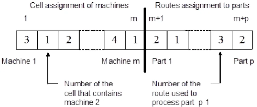
The cell formation problem is a crucial component of a cell production design in a manufacturing system, therefore, most researches proposed GAs to solve the grouping of parts and machines problem. For example, genetic algorithms have been applied to solve part-machine problems by Pierreval et al. (2003). This problem consists of grouping machines into cells and in determining part families such that parts of a family are entirely processed in one cell. A typical possible way to encode solutions (in other words representation) is to use a two-fold integer string. The first m positions of the string represent the assignment of the m machines, and the last p positions represent the assignment of the routes to the p parts. This coding is illustrated in Figure 1.

The grouping of parts and machines by genetic algorithm is also presented by Uddin and Shanker (2002). Their paper addresses generalized grouping problem where each part has more than one process routes. In this approach, the objective of minimization of intercell movements is achieved by minimizing the number of visits to various cells required by a process route for processing the corresponding part. The working of the proposed algorithm is illustrated with a numerical example and found that it can be a powerful tool for solving grouping problems.

Fig. 1 Coding of a solution (Pierreval, 2003)

Pailla et al. 2010 introduced a specialized evolutionary algorithm to solve the manufacturing cell formation problem. In their approach, the objective is to build manufacturing clusters by associating part families with machine cells, with the aim of minimizing the inter-cellular movements of parts by grouping efficacy measures. Considering the different approaches found in the literature for coding a CFP solution as a string of characters, they have used the proposal of Joines et al. (1996). In this encoding method, each individual is composed of (m + n) genes, where m is the number of machines and n is the number of parts of the problem. In this way, an individual is represented as s = (x1,…, xm  y1,…,yn). Every gene xi indicates

the cluster to which the ith machine is assigned, and every gene yi indicates the cluster

to which the ith part is assigned (Pailla et al. 2010). The study showed that the evolutionary algorithm proposed by authors is very effective.

A differential evolution algorithm for the manufacturing cell formation problem using group based operators was proposed by Noktehdan et al. (2010). In their study, the main objective of CF is to construct machine cells and part families, and then dispatch part families to machine cells to optimize the chosen performance measures such as inter-cell and intra-cell transportation cost, grouping efficiency and exceptional elements. The algorithm developed in this study (GDE) uses the encoding strategy, namely the grouping encoding which was proposed by (Falkenauer, 1992). The grouping encoding scheme uses a variable length

chromosome (solution) that includes the items to be grouped along with an additional section denoting the actual groups present in the solution. For example, consider the individual ABCB that encodes the solution where the first object is in group A, second in B, third in C, and fourth in B. The grouping encoding related to this individual could be ABCBBAC. Note that the order in which the groups are listed does not matter (the order BAC) (Falkenauer, 1992). This representation is crucial to the design of the GDE, as the modified operators for crossover and mutation are designed to manipulate the group portion of the individuals. The encoding scheme used for the machine–part cell formation (MPCF) problem is a natural adaptation of this strategy. The chromosome representation consists of three sections: one representing the parts, one representing the machines, and the additional group section that may be variable length (Brown and James, 2007). The individuals used for the MPCF problem can be represented as shown in (1) where pi denotes what group part i is assigned, for parts 1, . . . ,P; mj denotes what group machine j is assigned,

for machines 1, . . . ,M; and gk denotes the group numbers for groups 1… K

p1p2p3p4 … pp m1m2m3m4 … mM  g1g2g3g4 … gK

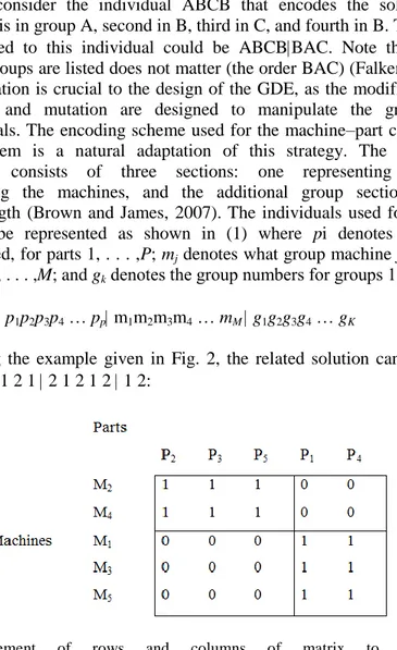
Considering the example given in Fig. 2, the related solution can be encoded as follows: 2 1 1 2 1  2 1 2 1 2  1 2:

Fig. 2 Rearrangement of rows and columns of matrix to create cells (Noktehdan et al., 2010)

For this example, there are five parts and five machines. The group portion of the individuals can vary in length depending on the number of cells into which the machines and parts are grouped. The solution consist of two cells with the cell 1 containing parts {2, 3,5} and machines {2, 4}, and cell 2 containing parts {1,4} and machines {1, 3, 5}. Note that the part and machine portions of the individuals are fixed in length based on the size of the problem. The result of experiments show that

the proposed by authors the grouping genetic algorithm based on the grouping representation is effective in solving machine–part cell formation problem.

A multiobjective optimization approach which was based on a genetic algorithm for solving the manufacturing cell formation problem was developed by Neto and Filho (2010). The objective of their paper is to propose a multiobjective approach to the cell formation problem considering performance measures of the manufacturing system. Three conflicting objectives are to be minimized, such as the mean of the work-in-process (WIP) with the cellular system, the mean of the intercell movements for a part and the total machine investment. In this approach, the Pareto optimality principle was adopted in this solution procedure. In this paper, a cellular manufacturing system is denoted as a collection of cells, which are heterogeneous sets of machines. With heterogeneous, it is meant that a cell may be composed of different machine types, vis-á -vis homogeneous cells, which are sets of machines from the same type. Any machines which are indistinguishable with regards to operation capabilities are called replicate machines. Therefore, it is understood that they share the same type. A solution is represented by an integer matrix X, in which row i corresponds to cell i, and its column j corresponds to machine type j, whereby an element xij represents

the number of replicate machines from type j in cell i (Fig. 3).

Fig. 3 An example of the solution representation (Neto and Filho, 2010)

Beside, Deljoo et al. (2010) proposed a genetic algorithm to solve dynamic cell formation (DCF) problem. The objective is to minimize the sum of the following costs: 1. Machine cost: The investment and amortization cost per period to procure machines. This cost is calculated based on the number of machines of each type used in the DCF for a specific period.

2. Operating cost: The cost of operating machines for producing parts. This cost depends on the cost of operating each machine type per hour and the number of hours required for each machine type.

3. Inter-cell material handling costs: The cost of transferring parts between cells, when parts cannot be produced completely by a machine type or in a single cell. This cost is incurred, when batches of parts have to be transferred between cells.

Inter-cell moves decrease the efficiency of cellular manufacturing (CM) by complicating production control and increasing material handling requirements and flow time.

4. Machine relocation cost: The cost of relocating machines from one cell to another between periods. In dynamic and stochastic production conditions, the best cell formation (CF) design for one period may not be an efficient design for subsequent periods. By rearranging the manufacturing cells, the CF can continue operating efficiently as the product mix and demand change.

However, there are some drawbacks with the rearrangement of manufacturing cells. Moving machines from cell to cell requires effort and can lead to the disruption of production.

A chromosome or feasible solution for DCF problem consists of four genes as follow:               K N Y X

1. The gene related to assignment of part operation to machine is named matrix [X]. X consists of P matrices as [X]HxOp(i) where P is the number of products;

H is the number of periods and Op(i) is the number of operations of part i.

2. The gene related to the assignment of part operation to cells is named matrix [Y]. Y consists of P matrices as [Y]HxOp(i) where P is the number of products;

H is the number of periods and Op(i) is the number of operations of part i.

3. The gene related to the number of machines being available in each cell is named matrix [N]. N consists of M matrices as

 

HxC

N where C is the number

of cells and H is the number of periods.

4. The gene related to the number of machines being moved in each cell or the number of machines being moved out, is named matrix [K]. K consists of M matrices as

 

HxC

K where C is the number of cells and H is the number of periods.

Obtained results showed that proposed GA is fast.

Arkat et al. 2011 proposed also an algorithm, namely the multi-objective genetic algorithm to solve the cell formation problems. In their approach, there are two main objectives. The first objective is to minimize the number of exceptional elements. This objective function tries to minimize the number of parts which are moved between cells. The second objective function is to minimize the number of voids (the number of zero elements inside cells). Based on this claim, the proposed model has two objective functions. The following notations are used in the proposed model:

Index sets:

i: ndex for parts (i = 1,2,. . . ,n) j: Index for machines (j = 1,2,. . . ,m) k: Index for cells (k = 1,2,. . . ,C)

Parameters:

m: Number of machines n: Number of parts C: Number of cells

Uk: Maximum number of machines in cell k

Lk: Minimum number of machines in cell k

    othewise machine on processing needs part if 1 0 j i a_ij Decision variables:     otherwise cell to assigned is machine if 0 1 j k Y_jk     otherwise 0 cell to assigned is part if i k X_ik 1

The model is presented as follows:

  

 











 

jk,X ,

Y  10 

The first objective function (Eq. (2)) minimizes the number of exceptional elements outside of the cells and the second one (Eq.(3)) minimizes the number of voids inside the cells. The first and the second constraints (Eqs.(4) and (5)) are to bound the number of machines in each cell between the predefined minimum and maximum cell sizes, respectively. The third constraint (Eq. (6)) ensures that each machine is assigned to a single cell. The forth constraint (Eq. (7)) indicates that each part is assigned to a single part family. The last constraint (Eq. (8)) illustrates that the proposed model is a binary model. Two variables Xik and Yjk

are multiplied in both objective functions and therefore, the objective functions are in nonlinear forms. The authors define the following new binary variable set to linearize the objective functions:

k , j , i Y X Z_ijk  _{ik jk} 

Consequently, the objective functions become as follows:

  

 



The below linear constraints should be added to the model to enforce the Eq. (9).

k , j , i Z Y X_ik  _jk2 _ijk 0  k , j , i Z Y X_ik  _jk  _ijk 0 

The first new constraint (Eq. (12)) ensures that if one of the primary binary variables takes a zero value, then their corresponding new variable takes a zero value as well. The second new constraint (Eq. (13)) ensures that if both primary variables take unit values, then their corresponding new variable takes a unit value as well. Because of the minimization form of the objective functions, if at least one of the primary binary variables takes a zero value then the objective functions enforce the new variable to take a zero value as well and hence, the first new constraint is unnecessary and can be eliminated from the model. Thus,

(8) (9) (10) (11) (12) (13)

the considered model has two variable sets; one for assigning parts to the part families and the other for assigning machines to the cells (Fig. 4).

PF1 PF2 … PFn C1 C2 … Cm

Fig. 4 The chromosome structure

Therefore, each chromosome has two distinguishable segments in which genes represent the cell number for their corresponding part or machine, respectively.

The presented numerical examples by authors illustrated that the proposed GA can find the whole set of the efficient solutions for the large-scale problems in a reasonable run time. The proposed algorithms can help the decision maker to choose one of the efficient solutions based on his or her priorities.

3. EVOLUTIONARY ALGORITHM IN OPTIMIZATION

OF THE FACILITIES LAYOUT

Evolutionary algorithms find an application in optimization of facilities layout (Kazerooni et al., 1997), (Azadivar and Wang, 2000), (Ponnambalan et al., 2001), (Muruganandaram et al., 2005). The problem in machine layout design is to assign machines to locations within a given layout arrangement such that a given performance measure is optimized.

El-Baz (2004) described a genetic algorithm (GA) to solve the problem of optimal facilities layout in manufacturing systems design so that material-handling costs are minimized. The paper considers the various material flow patterns of manufacturing environments of flow shop layout, flow-line layout (single line) with multi-products, multi-line layout, semi-circular and loop layout. The facility layout problem addressed here is the assignment of M machines to N locations in a manufacturing plant. During the manufacturing process, material flows from one machine to the next machine until all the processes are completed. The objective of solving the facility layout problem is therefore to minimize the total material handling cost of the system. To determine the material handling cost for one of the possible layout plans, the production volumes, production routings, and the cost table that qualifies the distance between a pair of machines/locations should be known. The following notations are used in the development of the objective function:

Fij amount of material flow among machines i and j (i,j = 1,2,.,M).

Cij unit material handling cost between locations of machines i and j (i,j =1,2,.,M).

Dij rectilinear distance between locations of machines i, and j

The total cost function is defined as: ij ij M i M j ijC D F c



The evaluation function considered in this paper is the minimization of material handling cost, which is the criterion most researchers prefer to apply in solving layout problems.

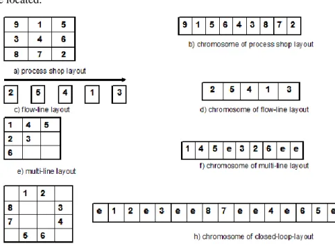
The technique of GAs requires a string representation scheme (chromosomes). In method of El-Baz (2004), the entire manufacturing plant/department is divided into N grids and each grid represents a machine location. In thisapproach, a form of direct representation for strings is used. Fig. 5 shows different examples of different types of production plant layout with their encoded chromosomes representation. This chromosome string representation indicates one of the possible machine layout plans of each production type. Examples of flow shop layout

containing nine machines/departments, production flow line contains

5 workstations, multi-line production system contains 6 machine locations, and a closed loop layout type of 8 machines are presented in the figure. The location assigned with the letter ‘e’ represented an empty area where no machine is allowed to be located.

Fig. 5 Types of layout and their chromosomes representation (El-Baz, 2004)

In recent years, GA has been proposed as an innovative approach to solve the dynamic plant layout problem. The dynamic problem involves selecting a static layout for each period and then deciding whether to change to a different layout in the next period. Balakrishnan et al. (2003) extend and improve the use of genetic algorithm by creating a hybrid GA for the dynamic plant layout problem. In this approach, the objective function is the sum of the material flow and the layout rearrangement costs for the planning horizon. The encoding scheme bases on scheme of Conway and Venkataramanan (1994). Each static layout is represented by a string and the concatenation of the static layout strings forms the dynamic layout string.. The study shows that the proposed algorithm iseffective

and it may be useful in solving the larger problems.

Solimanpur and Kamran (2010) applied genetic algorithm to solve the facilities layout problem in the presence of alternative processing routes using a genetic algorithm, where the chromosome consist of two segments. The first segment of the chromosome is made up of M genes and shows how M machines are located in M = L locations. The second segment is made up of P genes indicating the process selected for each product. For example, let us consider a problem with five products and eight machines to be located in eight locations. Suppose products 1, 2, 3, 4 and 5 have 5, 2, 3, 4 and 3 processing routes, respectively. A typical solution for this problem can be represented by the following chromosome. In this solution, machines 5, 7, 1, 8, 6, 2, 4 and 3 have been located in locations 1, 2, 3, 4, 5, 6, 7 and 8 respectively. Similarly, for products 1 to 5 the processing routes 2, 2, 1, 4 and 3 have been selected 5-7-1-8-6-2-4-3-2-2-1-4-3. It is worth noting that the aforementioned encoding scheme can yet be used for cases where L > M. To capture this case, a number of L–M virtual machines are to be assumed. For example, suppose there are three products and eleven machines to be located in fifteen locations. Therefore, four virtual machines numbered as 12, 13, 14 and 15 are assumed. A typical solution for this problem may be the following chromosome in which locations 3, 7, 10 and 14 are in fact empty 3-2-14-1-8-4-13-11-7-15-6-10-9-12-5-3-1-1. The effectiveness of the GA approach was evaluated with numerical examples. The results showed that the proposed GA is effective and efficient in solving the facilities location problem.

A=1 C=3 E=5 G=7

B=2 D=4 F=6 H=8

Fig. 6 Location (Yang et al., 2011)

A genetic algorithm for dynamic facility planning in job shop manufacturing was also proposed by Yang et al. (2011). Their study apply a genetic algorithm to solve the facility layout problem, considering the handling cost, the facility moving cost, and the facility setup cost. In this approach, each chromosome consists of a priority number and a randomly selected facility from the set of alternative facilities

for each location. For example, the chromosome (1, 2, 3, 4, 5, 6, 7, 8) denotes that each gene corresponding to the following locations in Fig. 6:

1A, 2B, 3C, 4D, 5E, 6F, 7G, 8H.

The computational results showed that the GA-based approach performs well.

4. GENETIC ALGORITHMS FOR LOT-SIZING PROBLEM

Recent works have shown that the calculation of lot-sizing through simulation optimization can be efficiently addressed using genetic algorithms. For example, Berretta and Rodrigues (2004) presented a memetic algorithm (MGA) to solve the multistage capacitated lot-sizing problem, considering setup time and setup cost

where a genetic algorithm hybridized with a local search procedure used

to intensify the search process. In this study, the lot-sizing problem is described as follows. In a multistage production system there are N items to be produced in T periods in a planning horizon such that a demand forecast would be attained. The planning of each item depends on the production of other items, which are situated at lower hierarchical levels. The resources for production and setup are limited. The lead times are assumed to be zero. Each solution is represented by a matrix of size 2 N x T (where N is number of items and T number of periods), with lot-size and inventory of each item in each period. The objective function is to minimize the sum of production, inventory and setup costs in T periods. The mathematical modeling is as follows. Let N be the number of types of items (I = 1,2, …, N), T the number of periods in the planning horizon (t = 1,2, …,T), K the number of types of resources (k = 1,2, …, K), cit the unit production cost

of item i in period t; hit the unit holding cost of item i in period t; sit the setup cost

of item i in period t; dit the demand (forecast) for item i in period t; vikt the unit

amount of resource k necessary to produce item i in period t; fikt the fixed amount

of resource k necessary to produce item i in period t; bkt the amount of resource

k available in period t; M an upper bound on xit; S(i) the set of immediate successor

items to item i; and rij is the number of units of item i needed by one unit of item

j; where j  S(i). The decision variables are: xit is the lot-size of item i in period

t; yit the 1 if item i is produced in period t and 0, otherwise. Iit is the inventory

of item I in period t. The mathematical formulation can be written as follows:















The objective function (1) is to minimize the sum of production, inventory and setup costs in T periods. Eq. (16) are the inventory balance constraints, constraints, which describe the relationship between inventory and production at the beginning and the end of the period. Constraints (17) represent the capacity limitation of production and setup. Constraints (18) ensure that the solution will have setup when it has production. The last two constraints (19) and (20) require that variables must be positive and the setup variables must be binary.

The MA provided a very useful strategy to obtain good results for the multistage capacitated lot-sizing, improving results obtained by other heuristics.

An adaptive genetic algorithm for lot-sizing problem was also presented by Hop and Tabucanon (2005). In this approach, the timing of replenishment is encoded as a string of binary digits (a chromosome). Each gene in that chromosome stands for a period. Standard GA operators are used to generate new populations. These populations are evaluated by a fitness function using the replenishment scheme of solution based on the total cost. Through this evaluation, the rates of GA operators for the next generation are automatically adjusted based on the rate of survivor offspring, which are generated by corresponding operators. The oriented search procedure using these self-adjustment rates of operator schemes can give faster and better solutions. Some experimental results confirm the theoretical judgment.

A successful application of the proposed a genetic algorithm to lot-sizing problem with supplier selection is also reported by Rezaei and Davoodi (2011).

5. ASSEMBLY LINE BALANCING PROBLEM

A well-known manufacturing optimization problem is the assembly line balancing problem (ALBP). Due to the complexity of the problem, in recent years, a growing number of researchers have employed genetic algorithms. ALBP deals with the allocation of the tasks among workstations so that the precedence relations are not violated and a given objective function is optimized.

Several versions of ALBP arise by varying the objective function. It is noted that the most commonly used objective function in the literature is the maximization of the line efficiency (Tasan and Tunali, 2008):

(17)

(18) (19) (18)

E = tsum/(n*c).

where

n - number of workstations; i=1,. . .,n

c - cycle time

m - number of tasks; j = 1,. . ., m

tj - processing time of task j

tsum - total processing time of tasks;



  m j j sum t t 1

The maximization of the line efficiency is the most general problem version, which tries to maximize the line efficiency by simultaneously minimizing the cycle time and a number of workstations.

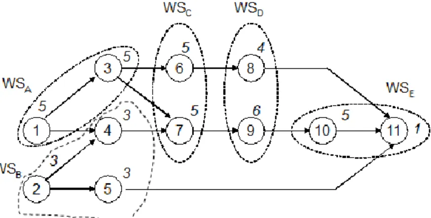
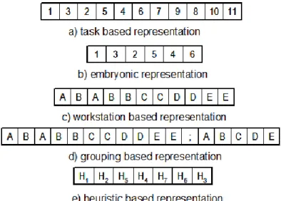
The first step in applying GA to a particular problem is to convert the solutions (individuals) of ALBP into a string type structure called chromosome. In a survey study on assembly line balancing, the Tasan and Tunali (2008) noted five different types of chromosome representation schemes; i.e. task based, embryonic, workstation based, grouping based, and heuristic based. Alternative chromosome representation schemes can be illustrated using the example given in Fig. 6, where the cycle time c, is 10min and number of workstations, n is 5. The workstation loads for this solution are WSA={1, 3}, WSB={2, 4, 5}, WSC={6, 7},WSD={8, 9}, and WSE={10, 11}.

Fig. 7 Signature under drawing

1. Task based representation: The chromosomes are defined as feasible precedence sequences of tasks (Sabuncuoglu et al., 2000). The length of the chromosome

is defined by the number of tasks. For example, the task based representation of the solution given in Fig. 7 is illustrated in Fig. 8a.

2. Embryonic representation: Embryonic chromosome representation that was proposed by Brudaru and Valmar (2004) is actually a special version of the task based chromosome. Only difference between the two is that the embryonic representation of a solution considers the subsets of solutions rather than the individual solutions. During the generations, the embryonic chromosome evolves through a full length solution. Therefore, the chromosome length varies throughout the generations. The length is initially defined by a random number and then increases until it reaches the number of tasks. Figure 8b illustrates an example of embryonic representation of the solution given in Fig. 8.

3. Workstation based representation: The chromosome is defined as a vector containing the labels of the workstations to, which the tasks are assigned (Kim et al., 2000). The chromosome length is defined by the number of tasks. For example, the workstation based representation of the solution given in Fig. 8 is illustrated in Fig. 8c, where the task 4 is assigned to workstation B.

Fig. 8 Chromosome representation schemes (Tasan and Tunali, 2008)

4. Grouping based representation: In grouping based representation, the workstations are represented by augmenting the workstation based chromosome with a group part (Falkenauer and Delchambre 1992). The group part of the chromosome is written after a semicolon to list all of the workstations in the current solution (see Fig. 8d). The length of the chromosome varies from solution to solution. As it is seen in Fig. 8d, the first part is the same

as in workstation based chromosome. Difference comes from the grouping part, which list all the workstations, i.e. A, B, C, D, and E.

5. Heuristic based (indirect) representation: This type of representation scheme represents the solutions in an indirect manner. Gonçalves and De Almedia (2002), and Bautista et al. (2000) coded the priority values of the tasks (or a sequence of priority rules), then they applied these rules to the problem to generate the solutions. The chromosome length is defined by the number of heuristics. For example, Fig. 8e shows an example chromosome having seven different heuristics, which are used in the sequence of H1, H2, H5, H4, H7, H6 and H3 to assign the tasks to the workstations.

Some researchers proposed evolutionary approach to the planning and scheduling assembly problem. For example, Perkoz et al. (2007) developed a multi-objective model to optimally control the lead time of a multi-stage assembly system, using genetic algorithms. The multi-stage assembly system is modeled as an open queueing network. They apply a genetic algorithm with double strings. According to the numerical experiments, it is seen that the genetic algorithm method is an efficient method for the multi-objective lead time control problem.

An interesting review of the applications of genetic algorithms in assembly line balancing has been published by Tasan and Tunali (2008).

6. OPTIMIZATION OF THE SUPPLY NETWORK

CONFIGURATION

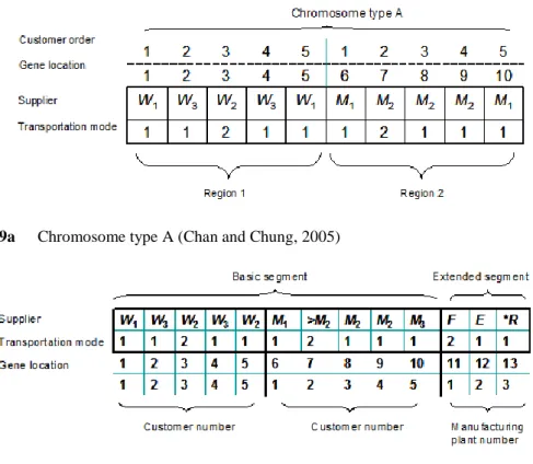
A crucial question in the supply chain is the design of distribution networks and the identification of facility locations (Liao et. Al 2011). Many researchers have studied optimization of distribution networks. Chan and Chung (2005) adopted GAs to minimize the total cost for a distribution network (i.e. the total lead time of demands, the total number of tardy demands, the total duration of tardiness time, and the mean absolute deviation of tardy demands). For enabling multicriterion decision-making, the proposed algorithm combines analytic hierarchy process with genetic algorithms (GAs). The problem is divided into two parts  (I) demand allocation and transportation problem, and (II) production scheduling problem. In this approach, as above mentioned, one of the objective functions is to minimize the total system cost. Other objective functions are to minimize the total lead time of demands, the total number of tardy demands, the total duration of tardiness time, and the mean absolute deviation of tardy demands. In this approach, each chromosome represents a potential optima solution of a problem being optimized. According to the problem structure, two different types of chromosomes are designed. Chromosome type A is designer for Part I. This chromosome is represented by a 2- dimensional matrix, as shown in

Figure 9a. In the supplier row, region 1, the value of gene represents the warehouse number, and the location of the gene represents the customer number. This implies that the corresponding demand will be supplied through the corresponding warehouse assigned.

In region 2, the value of gene represents the manufacturing plant number, and the location of the gene represents the customer number.

Fig. 9a Chromosome type A (Chan and Chung, 2005)

Fig. 9b Chromosome type B (Chan and Chung, 2005)

This implies that the corresponding demand will be produced

in the corresponding manufacturing plant allocated. With a similar interpretation, the transportation row shows the transportation mode to adopt.

In region 1, it indicates the transportation mode between the warehouse and customer for a particular demand. In region 2, it indicates the transportation mode between manufacturing plant and warehouse for a particular demand. Chromosome type B is designed for Part II, as shown in Figure 9b. The production scheduling row indicates the ranking number of demand in the production scheduling in its manufacturing plant assigned.

In recent years, GA has been proposed as an innovative approach to solve the configuration of the supply network. For example, a hybrid genetic algorithm

for multi-time period production/distribution was presented by Gen and Syarif (2005). They considered a production/distribution problem to determine an efficient integration of production, distribution and inventory system so that products are produced and distributed at the right quantities, to the right customers, and at the right time, in order to minimize system wide costs while satisfying all demand required. This problem was viewed as an optimization model that integrates facility location decisions, distribution costs, and inventory management for multi-products and multi-time periods. The authors presented a comprehensive mathematical model that considers real-world factors and constraints of the problem. The notations used in the model are defined as follows:

Indices

t index of time period (t=1,2,.,T) i index of product (i=1,2,.,I) j index of plant (j=1,2,.,J) k index of resource (k=1,2,.,K) m index of customer (m=1,2,.,M) Parameters

aijk amount of resource k required to produce one unit of product i at plant j

bjk(t) amount of resource k available at plant j in period t

dim(t) demand for product i by customer m in period t

pij(t) unit cost of production for product i at plant j in period t

qij(t) unit inventory holding cost for product i at plant j in period t

cijm(t) shipping cost of product i from plant j to customer m in period t

Variables

xij(t) amount of product i produced at plant j in period t

yij(t) inventory product i at plant j in period t

zijm(t) amount of product i shipped from plant j to customer m in period t

In this problem, the authors determined the production number for each product in each plant, inventory strategy and distribution network design to satisfy the resource capacity and customer demand with minimum cost. It can be formulated as follows: ) ( ) ( ) ( ) ( ) ( ) (t x t q t y t c t z t p min _ijm T t I i J j M m ijm ij T t I i J j T t t i J j ij ij ij









t , m , i , t d t z J j im ijm() () 





In the above model, the objective function captures production and inventory holding costs, which depend on the plant, plus transportation or distribution cost for shipment of product from plant to the customer. The constraint (23) is the inventory balance constraint that assures the supply of an item at each plant is either held in inventory or shipped to a customer to meet demand. Constraint (24) ensures that the shipments satisfy the demand of each customer for each period. Constraint (25) is a set of resource constraints. Production in each period is limited by the availability of a set of shared resources. Typical resources are various types of labor, process and material handling equipment and transportation modes.

To solve the problem, the authors proposed the technique called spanning tree-based genetic algorithm.

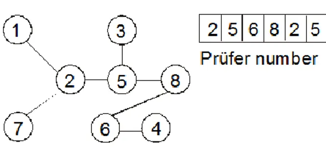
In the supply network optimization, the minimum spanning tree (MST) problem is great importance. This problem can be viewed as an optimization model that integrates facility location decision, distribution costs, and inventory management for multi-products and multi-periods (Gen and Syarif, 2005). The multi-criteria MST is a more realistic representation of the practical problem in the configuration of the supply net. The minimum spanning tree problem is to find a least-cost spanning tree in an edge-weighted graph. The proposed methods adopt the Prüfer number as the tree encoding. Prüfer describes a one-to-one mapping between spanning trees on n nodes and strings of n-2 nodes labels. The Prüfer number encoding procedure has the following major steps:

Step 1: Let vertex j be the smallest labeled leaf vertex in a labeled tree T.

Step 2: Set k to the first digit in the permutation if vertex k is incident to vertex j.

Step 3: Remove vertex j and the edge from j to k, we have a tree with n1 vertices.

Step 4: Repeat above steps until one edge is left and produce the Prüfer number or permutation with n  2 digits in order.

An example is given to illustrate this encoding (Zhou and Gen, 1999). The Prüfer number [2 5 6 8 2 5] corresponds to a spanning tree on 8-vertex complete graph represented in Fig. 10. The construction of the Prüfer number is described as follows: locate the leaf vertex having the smallest label. In this case, it is vertex 1. Since vertex 2 (the only vertex) is incident to vertex 1 in the tree,

(24)

(25)

assign 2 to the first digit in the permutation, then remove vertex 1 and edge (1,2). Now vertex 3 is the smallest labeled leaf vertex and vertex 5 is incident to it, assign 5 to the second digit in the permutation and then remove vertex 3 and edge (3,5). Repeat the process on the subtree until edge (5,8) is left and the Prüfer number of this tree with 6 digits is finally produced.

Fig. 10 A tree and its Prüfer number (Zhou and Gen, 1999)

In many published works (Chen et al., 2007), (Zhou et al., 2002), and (Syarif et al., 2002), a genetic algorithm approach is developed to deal with this problem. Recently, a new spanning tree-based genetic algorithm was developed by Wang and Hsu (2010), Hajiaghaei-Keshteli et al. (2010), and Ying-Hua (2010). The studies focus on the design of configuration and the transportation planning in multi-stage supply chain networks. The researches presented successful implementations of genetic algorithms.

7. EVOLUTIONARY ALGORITHMS FOR PRODUCTION

PLANNING AND SCHEDULING

A global supply network is usually characterized by a long time of transport and large size of operations. Therefore, it is not possible to create one common system for operation management in the global supply network. In this network, each node (i.e. enterprise) applies an autonomous method for operations management, and detailed production scheduling is performed individually for each plant. In the industrial cluster, there are transport operations with a relatively short time and a relatively smaller number of operations. In this supply network, the operations management can be executed together.

Planning and scheduling plays an important role to implement effective supply chain management methods. But its implementation would not be easy with the conventional information systems (Chang, 2007). Therefore, a short literature review on the adaptation of genetic algorithms to planning and scheduling is presented below.

Scheduling problem is an assignment problem, which can be defined as the assigning of available resources (machines) to the activities (operations) in such a manner that maximizes the profitability, flexibility, productivity, and performance of a production system (Prakash et al., 2011). The scheduling with makespan objective can be formulated as follows (Cheng et al.,1996):

 









where cjk is the completion time of job j on machine k, tjk is the processing time

of job j on machine k, M is a big positive number, aihk is an indicator coefficient

defined as follows:     otherswise 0 job for machine on that precedes machine on processing if 1 h k i a_ihk

and xijk is an indicator variable defined as follows:

    otherswise 0 machine on job precedes job if 1 i j k a_ihk

The objective is to minimize makespan. Constraint (28) ensures that the processing sequence of operations for each job corresponds to the prescribed order. Constraint (29) ensures that each machine can process only one job at the time.

As mentioned above, genetic algorithms work with a population of potential solution to a problem. A population is composed of chromosomes (i.e. a string), where each chromosome represents one potential solution. In ordering problem using the genetic algorithm, critical issue is developing a representation scheme to represent a feasible solution. A tutorial survey of job shop scheduling problem using different representation in genetic algorithm has been published by Cheng et al. (1996). During the last years, the following nine representations for the job-shop scheduling problem have been often proposed: operation-based representation, job-based representation, preference list-based representation,

(27)

(28) (29) (30) (31)

job pair relation-based representation, priority rule-based representation, disjunctive graph-based representation, completion time-based representation,

machine-based representation, random keys representation and others.

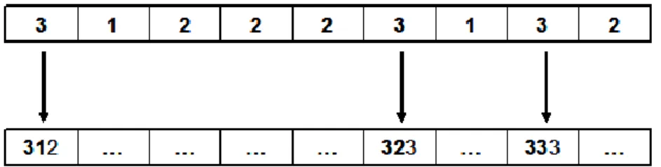
In the scheduling problem, the popular representation is operation-based method. This representation encodes a schedule as a sequence of operations and each gene stands for one operation. One natural way to name each operation is using a natural number. A schedule is decoded from a chromosome with the following decoding procedure (Cheng et al. 1996): (a) firstly translate the chromosome to a list of ordered operations; (b) then generate the schedule by a one-pass heuristic based on the list. The first operation in the list is scheduled first, then the second operation, and so on. Each operation is allocated in the best available time for the corresponding machine the operation requires. The process is repeated until all operations are scheduled. As an example, consider the 3-job 3-machine problem given in table 1.

Table 1 Example of 3-jobs and 3-machines

Job 1 2 3

Operation 1 2 3 1 2 3 1 2 3

Processing time 2 5 3 4 3 2 2 3 4

Machine 1 2 1 3 1 2 2 3 3

Suppose a chromosome is given as [3 1 1 2 2 3 1 3 2]. Each gene uniquely indicates an operation, and can be determined according to the order of occurrence in the sequence (Fig. 11).

Fig. 11 Operation-based representation

Let ojim denote the ith operation of job j on machine m. The chromosome can be

translated into a unique list of ordered operations of [o312 o111 o122 o213 o221 o323 o131

o333 o232]. Operation o312 has the highest priority and is scheduled first, then o111 ,

Fig. 12 Decoded active schedule

A huge amount of literature on scheduling, including the use of genetic algorithms, has been published within the last years. Most researchers proposed genetic algorithms to solve the flow shop scheduling problem. In these works, the objective was often to minimize the makespan. For example, Chang et al. (2005) proposed a two-phase sub-population genetic algorithm to solve the parallel machine-scheduling problem. The algorithm is divided into two phases. The first phase applies subpopulations, which concentrates on specific search space and prevents all individuals from converging to a local optimal. Then, in order to explore the solution space ignored or missed in the first phase, sub-populations are regrouped as a single big population. Each individual chromosome in this big population of the second phase is randomly assigned a weight value to explore more of the solution space. Experimental results are reported and the superiority of this approach is discussed. An evolutionary algorithm for scheduling a flowshop manufacturing cell with sequence dependent family setups has been also suggested by França et al. (2005). They proposed evolutionary heuristic algorithms to minimize the makespan in a pure flowshop manufacturing cell problem with sequence dependent setup times between families of jobs. The heuristic algorithms implemented are a Memetic Algorithm (MA), a Genetic Algorithm (GA) and a Multi-Start (MS) strategy. Computational results show that the proposed algorithms are relatively more effective in minimizing the makespan than the best known heuristic algorithm. The performance of the three proposed heuristic algorithms was very similar, with a slight superiority demonstrated by the memetic implementation. The flowshop scheduling problem with the objective of minimizing makespan was developed by Ruiz and Maroto (2006). They developed a genetic algorithm for hybrid flowshops with sequence dependent setup times and machine eligibility. Numerical computation based on benchmarks demonstrated the effectiveness of the proposed method. An improved genetic algorithm with the objective of minimizing the makespan for the flow shop scheduling problem was also proposed by Rajkumar and Shahabudeen (2009). Numerical computation based on benchmarks demonstrated the effectiveness of the proposed method.

Recently, some genetic algorithms have been developed for the multi-objective flow shop problem. For example, Arroyo and Armentano, 2005 presented a multi-objective genetic local search algorithm, which was applied to multi-multi-objective flow shop problems in order to find an approximation of the Pareto optimal set. The algorithm is applied to the flow shop scheduling problem for the following two pairs of objectives: (i) makespan and maximum tardiness; (ii) makespan and total tardiness. Computational results show that the proposed algorithm yields a reasonable approximation of the Pareto optimal set.

Onwubolu and Davendra (2006) presented a differential evolution algorithm for the flow shop scheduling problem in which makespan, mean flowtime, and total tardiness are the performance measures. From experimentation, the differential evolution algorithm is found to perform better than the genetic algorithm for small-sized problems, and competes appreciably with the genetic algorithm for medium to large-sized problems.

The job-shop scheduling problem (JSSP) is one of the most general and difficult of all traditional scheduling problems (Li and Chen, 2011). Many different approaches have been applied to JSSP and a rich harvest has been obtained. A genetic algorithm for job shop scheduling problems with alternative routings was proposed by Moon et al. (2008). In this approach, the chromosome is composed of two parts. The first part is for the assignment of alternative machines, and the second part is the relative processing order between jobs. The length of each chromosome is equal to the total number of operations. This genetic algorithm generated relatively good solutions quickly.

Currently, there is a research trend in the adaptation of hybrid approaches which combine different concepts or components of various techniques. The trends have been presented by Kobbacy, et al. (2007) in a very interesting survey of applications of artificial intelligence techniques for operations management. They reported that several authors use genetic algorithms to carry out an intelligent search by proposing alternative schedules and then using neural network to asses the quality and fitness of the schedule. Besides, fuzzy logic and genetic algorithms have been combined effectively for scheduling. A hybrid of genetic algorithm and bottleneck shifting for multiobjective flexible job shop scheduling problems (fJSP) was presented by Gao et al. (2007). They developed a new genetic algorithm hybridized with an innovative local search procedure (bottleneck shifting) for the problem. The fJSP problem is a combination of machine assignment and operation scheduling decisions. A solution can be described by the assignment of operations to machines and the processing sequence of operations on the machines. Because the genetic algorithm uses two representation methods to depict solution candidates of the fJSP problem, the chromosome is composed of two parts: machine assignment vector and operation sequence vector. The simulation results obtained by the authors are compared with those obtained by other methods. The genetic algorithm generated relatively good solutions. A hybrid genetic

algorithm was also developed by Chen et al. (2008) for the re-entrant flow-shop scheduling problem (RFS). In a RFS, all jobs have the same routing over the machines of the shop and the same sequence is traversed several times to complete the jobs. The aim of this study is to minimize the makespan by using the genetic algorithm (GA) to move from the local optimal solution to the near optimal solution for RFS scheduling problems. For the job shop scheduling problem, a hybrid evolutionary algorithm was also presented in work of Zobolas et al., (2009). In their work, the optimization criterion is minimization of the makespan and the solution method consists of three components: a Differential Evolution-based algorithm to generate a population of initial solutions, a Variable Neighbourhood Search method and a Genetic Algorithm to improve the population, the latter two are interconnected. Computational experiments on benchmark data sets demonstrate that the proposed hybrid metaheuristic reaches high quality solutions in short computational times using fixed parameter settings. Besides, a hybrid approach with an expert system and a genetic algorithm to production management in supply network was also presented by Ławrynowicz (2006, 2007).

Genetic algorithms have been successfully implemented to solve various planning and scheduling problems. For example, Lee et al., (2002) developed advanced planning and scheduling with outsourcing in manufacturing supply chain. The proposed model considers alternative processes plans for different job types. Chen and Ji (2007) proposed a genetic algorithm for dynamic advanced planning and scheduling with frozen interval. This paper investigates a dynamic advanced planning and scheduling (DAPS) problem where new orders arrive on a continuous basis. A periodic policy with a frozen interval is adopted to increase stability on the shop floor. A genetic algorithm is developed to find a schedule such that both production idle time and penalties on tardiness and earliness of both original orders and new orders are minimized at each rescheduling point. The numerical results confirm that the proposed methodology can improve the schedule stability while retaining efficiency.

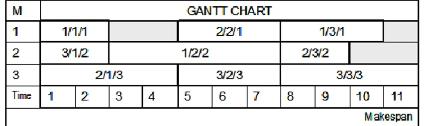
Few researchers have considered methods with genetic algorithms to support scheduling in distribution manufacturing systems. For example, Chan et al., 2005 proposed an optimization algorithm named Genetic Algorithm with Dominated Genes (GADG) to solve distributed production scheduling problems with alternative production routings. GADG implements the idea of adaptive strategy. In this paper, a new crossover mechanism named dominated gene crossover has been introduced to enhance the performance of genetic search, and eliminate the problem of determining an optimal crossover rate. A number of experiments have been carried out. The results indicate that significant improvement could be obtained by the proposed algorithm. An integration of the genetic algorithm and Gantt chart (GC) for job shop scheduling in distributed manufacturing systems has been also proposed by Jia et al., 2007. The integration of GA–GC is shown to be efficient at solving small-sized or medium-sized scheduling problems for

a distributed manufacturing system. Multiple objectives can be achieved, including minimizing the makespan, job tardiness, or manufacturing cost.

Application of the genetic approach for advanced planning in multi-factory environment is presented in the work of Chung et al. 2010. The proposed algorithm adopts the idea of dominant gene in the crossover operation proposed by Chan et al. (2005). The model is subject to capacity constraints, precedence relationships, and alternative machines with different processing time. The objective function is to minimize the makespan, which consists of the processing time, the transportation time between resources either within the same factory or across two different factories, and the machine set-up time among operations. The results show the robustness of the proposed algorithm for this problem.

As shown above, despite many advantages in solving scheduling problems with genetic algorithms, the application of the above mentioned algorithms is questionable. Frequently, the loops in supply networks are not taken into consideration in many works.

A modern hybrid approach for control problems in a node of supply network was published by Ławrynowicz (2008). This approach takes into account the loops in supply networks. In this approach, the production planning problem is first solved, and then the scheduling problem is considered within the constraints of the solution. The main objectives of this approach are to produce an Advanced Production Management (APRM) model that minimizes the makespan by considering alternative machines, alternative sequences of operations with precedence constrains, and outsourcing.

Summarizing, advances in genetic algorithms create new prospects for inter-organizational cooperation. It is common knowledge that in solving large-size problems, genetic algorithms show much better performance (Chung et al., 2010). Despite many advantages in solving scheduling problems presented in the existing literature, many applications of genetic algorithms are questionable. As mentioned above, researchers still study small-scale problems or only flow shop problems (Zhang et al., 2011), where there are many constraints. Many genetic algorithms proposed in the literature have been created for scheduling in a single factory. The approach often ignores dividing jobs and interactions between the various firms within supply networks at operations management level in order to improve manufacturing processes. In the era of supply network, decisions on the use of resources should concern both internal and external capacities; the internal flow of materials should be synchronized with the incoming and outgoing flows. For this purpose, a system for scheduling must take into consideration the possibility of dividing jobs into factories, loops, and a long transport. Therefore, the author proposed modified genetic algorithm (MGA), which take into account loops in supply networks Ławrynowicz (2009, 2010). Additionally, the proposed modified genetic algorithm enables dividing jobs between factories, and transport orders planning in the industrial cluster. The algorithm