L-statistics as Nonparametric Quantile Estimators
Ryszard Zieli´nskiInstitute of Mathematics, Polish Acad.Sc. POBox 21, Warszawa 10, Poland
e-mail: R.Zielinski@impan.gov.pl
Key Words: quantiles, Harrell-Davis estimator, Kaigh-Cheng estimator; L-statistics; optimal estimation.
Introduction
The basic nonparametric model in this note is a statistical model with the family
F of all continuous and strictly increasing distribution functions. In abundant literature
of the subject, there are many proposals for nonparametric estimators of quantiles, for example simple order statistics or convex combination of two consecutive order statistics [Davis and Steinberg (1986)], some more sophisticated L-statistics such as Harrell and Davis (1982) or Kaigh and Chen(1991), etc. Asymptotically the estimators do not differ substantially but if the sample size n is fixed, which is the case of our concern, differences may be serious. It appears that in the nonparametric statistical model with the family F of possible distributions nontrivial L-statistics (the L-statistics which are not single order statistics) are highly unsatisfactory. For example [Zieli´nski 1995)] take the well known estimator of the median m(F ) of an unknown distribution F ∈ F from a sample of size 2n, defined as the arithmetic mean of two central observations M2n = (Xn:2n + Xn+1:2n)/2.
Let M ed(F, M2n) denote a median of the distribution of the statistic M2n if the sample
comes from the distribution F . Then for every C > 0 there exists F ∈ F such that
A numerical study (simulations)
To demonstrate that L-statistics are useless for estimating quantiles in the nonpara-metric model F with all continuous and strictly increasing distribution functions we decided to present the problem of estimating the median of an unknown F ∈ F with the following well known estimators:
Davis and Steinberg (1986)
X(n+1)/2:n, if n is odd; Xn/2:n+ Xn/2+1:n/2, if n is even,
Harrell and Davis (1982)
HD = n! [(n−12 )!]2 n X j=1 "Z j/n (j−1)/2[u(1 − u)] (n−1)/2du # Xj:n,
Kaigh and Cheng (1991) for n odd
KC = 2n1−1 n n X j=1 n−3 2 + j n−1 2 3n−1 2 − j n−1 2 Xj:n.
As the distributions for studying our problem we have chosen
Pareto with cdf
1 − x1α, x > 1, heavy tails, no moments of order k ≥ α,
Power (special case of Beta) with cdf
xα, x ∈ (0, 1), no tails, all moments ,
Exponential with cdf
If T is an estimator of the quantile xq(F ) of order q ∈ (0, 1) of an unknown distribution
F ∈ F then assessing the quality of the estimator in terms the bias EFT − xq(F ), Mean
Square Error EFT − xq(F ) 2
, etc, is impossible because the moments of F ∈ F may not exist.
We decided to study the differences bF(T ) = M ed(F, T ) − xq(F ), where M ed(F, T ) is
a median of estimator T if the sample comes from the parent distribution F . The quantity
bF(T ) is known as the bias in the sense of median, or median-bias, or shortly bias in
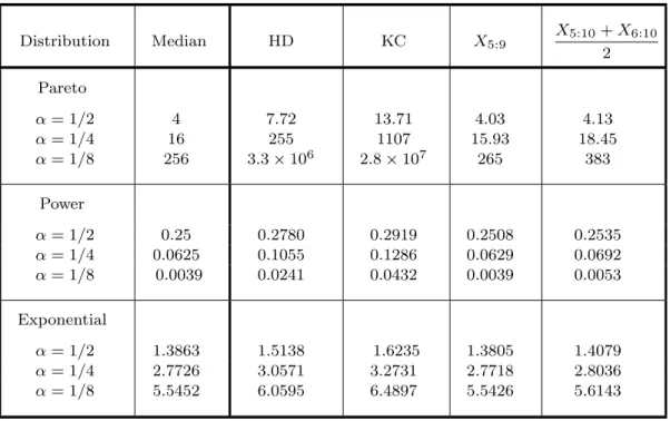
this note. Observe that M ed(F, T ) always exists and is finite. Results of our numerical investigations for samples of size n = 9 (Harrell-Davis, Kaigh-Cheng, and Davis-Steinberg statistic X5:9) or for samples of size n = 10 (Davis-Steinberg statistic (X5:10 + X6:10)/2)
are presented in Table 1. The number of simulated samples, and consequently the number of simulated values of the estimator under consideration, was N = 9, 999, and the median from the sample of size N = 9, 999 has been taken as an estimator of the median of the distribution of the estimator under consideration.
Table 1. Medians of estimators (simulated)
Distribution Median HD KC X5:9 X5:10+ X6:10 2 Pareto α = 1/2 4 7.72 13.71 4.03 4.13 α = 1/4 16 255 1107 15.93 18.45 α = 1/8 256 3.3 × 10⁶ 2.8 × 10⁷ 265 383 Power α = 1/2 0.25 0.2780 0.2919 0.2508 0.2535 α = 1/4 0.0625 0.1055 0.1286 0.0629 0.0692 α = 1/8 0.0039 0.0241 0.0432 0.0039 0.0053 Exponential α = 1/2 1.3863 1.5138 1.6235 1.3805 1.4079 α = 1/4 2.7726 3.0571 3.2731 2.7718 2.8036 α = 1/8 5.5452 6.0595 6.4897 5.5426 5.6143
To assess the exactness of the simulation we may compare columns ”Median” and ”X5:9”;
the latter is an unbiased estimator of the median so that the entries of both columns should be approximately equal.
It seems however that absolute differences bF(T ) = M ed(F, T )−xq(F ) are not suitable
measures of quality of an estimator (is the bias of HD really smaller when estimating median of the Power distribution than that for Exponential distribution?)
To ”normalize” the bias we may argue as follows. If T is an estimator of the qth quantile xq(F ) then F (T ) may be considered as an estimator of the (known!) value q (see
Figure 1). 0.0 1.0 ... ... ... ... ... ... ... ... ... ... ... ... ... ... ... ... ... ... ... ... ... ... ... ... ... ... ... ... ... ... ... ... ... ... ... ... ... ... ... ... ... ... ... ... ... ... ... ... ... ... ... ... ... ... ... ... ... ... ... ... ... ... ... ... x F (x) Figure 1 q xq(F ) T F (T ) = F (T0) T0
”Normalized” medians M ed(F, F (T )) are presented in Table 2. Now for every F ∈ F the median of F (T ) is obviously equal to q = 0.5 and differences between the entries of column
X5:9 and q = 0.5 illustrate the exactness of the results of simulations.
Table 2. F–medians of estimators (simulated)
Distribution Median HD KC X5:9 X5:10+ X6:10 2 Pareto α = 1/2 0.5 0.6401 0.7299 0.5016 0.5132 α = 1/4 0.5 0.7498 0.8265 0.4995 0.5175 α = 1/8 0.5 0.8471 0.8830 0.5022 0.5245 Power α = 1/2 0.5 0.5272 0.5403 0.5008 0.5035 α = 1/4 0.5 0.5700 0.5988 0.5008 0.5128 α = 1/8 0.5 0.6276 0.6752 0.5004 0.5197 Exponential α = 1/2 0.5 0.5308 0.5559 0.4986 0.5054 α = 1/4 0.5 0.5343 0.5588 0.4999 0.5039 α = 1/8 0.5 0.5319 0.5557 0.4998 0.5043
Theoretical results
A general result concerning the bias bF(T ) of estimation of the median m(F ) of an unknown
distribution F ∈ F is given in the following Theorem 1.
Theorem 1. Let T be the Harrell-Davis, or Kaigh-Cheng, or any L-estimatorPnj=1λjXj:n
such that λn > 0. Then for every C > 0 there exists a distribution F ∈ F such that
Proof. Observe that T ≥ λnXn:n a.s. and in consequence M ed(F, T ) ≥ λnM ed(F, Xn:n).
Consider the family
FM,α(x) = x − 1
M − 1
1/α
, 1 < x < M, M > 1, α > 0.
The median of the distribution is
m(FM,α) = 1 + (M − 1)2−α
The distribution function of Xn:n is FM,αn (x) and the median of that distribution is
M ed(FM,α, Xn:n) = 1 + (M − 1)2−α/n Now M ed(FM,α, T ) − m(FM,α) ≥ λnM ed(FM,α, Xn:n) − m(FM,α) = (M − 1)hλn2−α/n− 2−α i − (1 − λn) Choosing any α > − n
n − 1Log2λn (then λn2−α/n− 2−α is positive) and any M satisfying
M > 1 + C + (1− λn)
λn2−α/n− 2−λ
we obtain M ed(FM,α, T ) − m(FM,α) > C.
A general result concerning the bias of F (T ) when estimating a quantile of any order
q ∈ (0, 1) may be easily concluded from the following bounds for Med(F, F (T ).
Theorem 2. If T = Pmj=kλjXj:n is an L-statistic such that λk > 0, λm > 0, and
λk+ λk+1+ . . . + λm = 1, then
m(Uk:n) ≤ MedF, F (T )≤ m(Um:n)
where m(Uk:n) and m(Um:n) are the medians of order statistics Uk:nand Um:n from a
sam-ple of size n from the uniform U (0, 1) parent distribution. The bounds are sharp in the
Proof. The first statement follows easily from the fact that Xk:n < T < Xm:n and
hence for every F ∈ F we have Uk:n = F (Xk:n) < F (T ) < F (Xm:n) = Um:n. To prove the
second part of the theorem it is enough to construct families of distributions Fα, α > 0,
and Gα, α > 0, such that M ed(Fα, Fα(T )) → m(Um:n) and M ed(Gα, Gα(T )) → m(Uk:n),
as α → 0.
Consider the family of power distributions Fα(x) = xα, 0 < x < 1, α > 0. Then
Xj:n= Fα−1(Uj:n) = Uj:n1/α and Fα(T ) = λkUk:n1/α+ λk+1Uk+1:n1/α + . . . + λm−1Um−1:n1/α + λmUm:n1/α α = Um:n h λk Uk:n Um:n 1/α + λk+1 Uk+1:n Um:n 1/α + . . . + λm−1 Um−1:n Um:n 1/α + λm iα
If α → 0 then Fα(T ) → Um:n and M ed(Fα, Fα(T ))→ m(Um:n).
Now consider the family Gα with Gα(x) = 1− (1 − x)α; in full analogy to the above
we conclude that then Gα(T )→ Uk:n and M ed(Gα, Gα(T )) → m(Uk:n) as α → 0.
Example. For any estimator T =Pni=1λiXi:n with λ1, λn> 0, for n = 9 we have
0.074 ≤ Med(F, F (T )) ≤ 0.926
Note that the bounds do not depend of the order q of the quantile to be estimated. It follows that the normalized bias M ed(F, F (T )) − q of the estimator when estimating a quantile of order close to zero may be close to 0.926. By Theorem 1 the absolute bias
M ed(F, T )) − xq(F ) may be arbitrarily large.
Conclusions
A reason for the strange behavior of nontrivial L-statistics as quantile estimators is that they are not equivariant under monotonic transformation of data while the class F of all continuous and strictly increasing distribution functions is closed under such transfor-mations: if X is a random variable with distribution F ∈ F and g is any strictly monotonic transformation then the distribution of g(X) also belongs to F. The class of all statis-tics which are equivariant with respect to monotonic transformations of data is identical
with the class of all order statistics XJ:n, where J is a random index: P{J = j} = pj,
pj ≥ 0, Pnj=1pj = 1. Observe that if the sample comes from a distribution F ∈ F then
F (XJ:n) = UJ:n and the distribution of F (XJ:n) does not depend of a specific F ∈ F.
In the tables above only X5:9 is an equivariant statistic. It appears that in the large
nonparametric statistical model with the class F of all continuous and strictly increasing distribution functions the only reasonable estimators of quantiles are single order statistics
XJ:n with suitably chosen random index J. The index may bo chosen in such a way that
F (XJ:n) is an estimator of q which is uniformly minimum variance unbiased, or minimizes
Mean Square Error, or minimizes Mean Absolute Error, etc. (Zieli´nski 2004).
References
Davis, C.E. and Steinberg, S.M. (1986), Quantile estimation, In Encyclopedia of Statistical
Sciences, Vol. 7, Wiley, New York
Harrell, F.E. and Davis, C.E. (1982), A new distribution-free quantile estimator, Biometrika 69, 635-640
Kaigh, W.D. and Cheng, C. (1991): Subsampling quantile estimators and uniformity cri-teria. Commun. Statist. Theor. Meth. 20, 539-560
Zieli´nski, R. (1995), Estimating Median and Other Quantiles in Nonparametric Models.
Applicationes Math. 23.3, 363-370. Correction: Applicationes Math. 23.4 (1996) p. 475
Zieli´nski, R. (2004), Optimal quantile estimators. Small sample approach. IMPAN, Preprint 653, November 2004. Available at www.impan.gov.pl/˜rziel