Ryszard Zieli´
nski
OPTIMAL QUANTILE ESTIMATORS
SMALL SAMPLE APPROACH
Contents
1. The problem
2. Classical approach
2.1. Order statistics
2.2. Local smoothing
2.3. Global smoothing
2.4. Kaigh-Lachenbruch estimator
2.5. Comparisons of estimators
3. Optimal estimation
3.1. The class of estimators
3.2. Criteria
3.3. Optimal estimators
3.3.1. The most concentrated estimator
3.3.2. Uniformly Minimum Variance Unbiased Estimator
3.3.3. Uniformly Minimum Absolute Deviation Estimator
3.3.4. Optimal estimator in the sense of Pitman’s Measure of Closeness
3.3.5. Comparisons of optimal estimators?
4. Applications to parametric models
4.1. Median-unbiased estimators in parametric models
4.2. Robustness
4.2.1. Estimating location parameter under ε-contamination
4.2.2. Estimating location parameter under ε-contamination with restrictions
on contaminants
4.3. Distribution-free quantile estimators in parametric models; how much
do we lose?
5. Optimal interval estimation
6. Asymptotics
1
The Problem
The problem of quantile estimation has a very long history and abundant literature:
in out booklet we shall quote only the sources which we directly refer to.
We are interested in small sample and nonparametric quantile estimators.
”Small sample” is here used as an opposite to ”asymptotic” and it is meant that
the statistical inference will be based on independently and identically distributed
observations X
1
, . . . , X
n
for a fixed n. A short excursion to asymptotics is presented
in Chapter 6.
”Nonparametric” is here used to say that observations X
1
, . . . , X
n
come from an
unknown distribution F ∈ F with F being the class of all continuous and strictly
increasing distribution functions and, for a given q
∈ (0, 1), we are interested in
estimating the qth quantile x
q
= x
q
(F ) of the distribution F . If q is fixed (for
example, if we are interested in estimating the median only), the conditions for F
may be relaxed and F may be considered as the class of all locally at x
q
continuous
and strictly increasing distributions; we shall not exploit this trivial comment. The
nonparametric class F of distributions is rather large and one can hardly expect to get
many strict mathematical theorems which hold simultaneously for all distributions
F ∈ F. An example of such a theorem is the celebrated Glivenko–Cantelli theorem
for the Kolmogorov distance sup
|F
n
− F |. It appears that the class F is too large
to say something useful concerning the behavior of L-estimators; classical estimators
and their properties are discussed in Chapter 2. The natural class of estimators in F
is the class T of estimators which are equivariant under monotonic transformations of
data; under different criteria of optimality, the best estimators in T are constructed
in Chapter 3.
Our primary interest is optimal nonparametric estimation. Constructions of optimal
estimators are presented in Chapter 3 followed by their applications to parametric
models (Chapter 4) and some results concerning their asymptotic properties
(Chap-ter 6). An excursion to optimal in(Chap-terval estimation is presented in Chap(Chap-ter 5. In
Chapter 3 to Chapter 6 we present almost without changes previous results of the
author published since 1987 in different journals, mainly in Statistics, Statistics and
Probability Letters, and Applicationes Mathematicae (Warszawa).
Observe that in the class F of distributions, the order statistic (X
1:n
, . . . , X
n:n
), where
X
1:n
≤ . . . , ≤ X
n:n
, is a complete minimal sufficient statistic. As a consequence we
confine ourselves to estimators which are functions of (X
1:n
, . . . , X
n:n
). Some further
restrictions for the estimators will be considered in Chapter 3. We shall use T (q) or
shortly T as general symbols for estimators to be considered; the sample size n is
fixed and in consequence we omit n in most notations.
2
Classical Approach (inverse of cdf)
For a distribution function F , the qth quantile x
q
= x
q
(F ) of F is defined as x
q
=
F
−1
(q) with
(1)
F
−1
(q) = inf
{x : F (x) ≥ q}.
For F ∈ F and q ∈ (0, 1) it always exists and is uniquely determined. The well
recognized generalized method of moments or method of statistical functionals gives
us formally
(2)
T (q) = F
n
−1
(q) = inf {x : F
n
(x) ≥ q}
as an estimator T (q) of x
q
; here F
n
is an empirical distribution function. Different
definitions of F
n
lead of course to different estimators T . One can say that the variety
of definitions of F
n
(left- or right-continuous step functions, smoothed versions, F
n
as
a kernel estimator of F , etc) is what produces the variety of estimators to be found in
abundant literature in mathematical statistics. We shall use the following definition
of the empirical distribution function:
(3)
F
n
(x) =
1
n
n
X
i=1
1
(
−∞,x]
X
i
,
where the indicator function
1
(−∞,x]
X
i
= 1 if X
i
≤ x and = 0 otherwise. Note that
under the definition adapted, the empirical distribution function is right-continuous.
There are two kinds of estimators widely used. Given a sample, if F
n
(x) is a step
function then estimator (2) as a function of q ∈ (0, 1) takes on a finite number of
different values, typically the values of order statistics from the sample; if F
n
(x) is
continuous and strictly increasing empirical distribution function, so is its inverse
Q
n
(t) = F
n
−1
(t), t
∈ (0, 1), the quantile function, and T (q) can be considered as a
continuous and strictly increasing function of q ∈ (0, 1). An example give us
esti-mators presented in Fig. 2.2.1 (Sec. 2.2). In what follows we discuss both types of
estimators.
A natural problem arises how one can assess quality of an estimator, compare
distri-butions, or at least some parameters of distributions of different estimators of a given
quantile, or even the distributions of a fixed estimator under different parent
distri-butions F from the large class
F? In other words: how one can assess the quality of
an estimator in very large nonparametric class F of distributions? No characteristics
like bias (in the sense of mean), mean square error, mean absolute error, etc, are
acceptable because not for all distributions F ∈ F they exist or if exist they may be
infinite.
What is more: it appears that the model
F is so large that assessing the quality of
an estimator T of the q-th quantile x
q
(F ) in terms of the difference T − x
q
(F ) makes
no sense. To see that take as an example the well known estimator of the median
m
F
= x
0.5
(F ) of an unknown distribution F ∈ F from a sample of size 2n, defined
as the arithmetic mean of two central observations M
2n
= (X
n:2n
+ X
n+1:2n
)/2. Let
M ed(F, M
2n
) denote a median of the distribution of M
2n
if the sample comes from
the distribution F .
Theorem 1 (Zieli´
nski 1995). For every C > 0 there exists F ∈ F such that
M ed(F, M
2n
) − m
F
> C.
Proof . The proof consists in constructing F ∈ F for a given C > 0. Let F
0
be the
class of all strictly increasing continuous functions G on (0, 1) satisfying G(0) = 0,
G(1) = 1. Then F is the class of all functions F satisfying F (x) = G((x − a)/(b − a))
for some a and b (
−∞ < a < b < +∞), and for some G ∈ F
0
.
For a fixed t ∈ (
1
4
,
1
2
) and a fixed ε ∈ (0,
1
4
), let F
t,ε
∈ F
0
be a distribution function
such that
F
t,ε
1
2
=
1
2
,
F
t,ε
(t) =
1
2
− ε,
F
t,ε
(t
−
1
4
) =
1
2
− 2ε,
F
t,ε
(t +
1
4
) = 1 − 2ε.
Let Y
1
, Y
2
, . . . , Y
2n
be a sample from F
t,ε
. We shall prove that for every t
∈ (
1
4
,
1
2
)
there exists ε > 0 such that
(4)
M ed
F
t,ε
,
1
2
(Y
n:2n
+ Y
n+1:2n
)
≤ t.
Consider two random events:
A
1
= {0 ≤ Y
n:2n
≤ t, 0 ≤ Y
n+1:2n
≤ t},
A
2
= {0 ≤ Y
n:2n
≤ t −
1
4
,
1
2
≤ Y
n+1:2n
≤ t +
1
4
},
and observe that A
1
∩ A
2
= ∅ and
(5)
A
1
∪ A
2
⊆ {
1
2
(Y
n:2n
+ Y
n+1:2n
)
≤ t}.
If the sample comes from a distribution G with a probability density function g, then
the joint probability density function h(x, y) of Y
n:2n
, Y
n+1,2n
is given by the formula
h(x, y) =
Γ(2n + 1)
Γ
2
(n)
G
n−1
(x) [1 − G(y)]
n−1
g(x)g(y),
0
≤ x ≤ y ≤ 1,
and the probability of A
1
equals
P
G
(A
1
) =
Z
t
0
dx
Z
t
x
dy h(x, y).
Using the formula
Γ(p + q)
Γ(p)Γ(q)
Z
x
0
t
p−1
(1 − t)
q−1
dt =
p+q−1
X
j=p
p + q − 1
j
x
j
(1 − x)
p+q−1−j
,
we obtain
P
G
(A
1
) =
2n
X
j=n+1
2n
j
G
j
(t) (1 − G(t))
2n−j
.
For P
G
(A
2
) we obtain
P
G
(A
2
) =
Z
t−
140
dx
Z
t+
1 4 1 2dy h(x, y)
=
2n
n
G
n
(t
−
1
4
)
1 − G
1
2
n
−
1 − G(t +
1
4
)
n
.
Define C
1
(ε) = P
F
t,ε(A
1
) and C
2
(ε) = P
F
t,ε(A
2
). Then
C
1
(ε) =
2n
X
j=n+1
2n
j
(
1
2
− ε)
j
(
1
2
+ ε)
2n−j
,
C
2
(ε) =
2n
n
(
1
2
− 2ε)
n
1
2
n
− (2ε)
n
.
Observe that
C
1
(ε) %
1
2
−
1
2
2n
n
1
2
2n
as ε & 0
and
C
2
(ε)
%
2n
n
1
2
2n
as
ε
& 0.
Let ε
1
> 0 be such that
(∀ε < ε
1
)
C
1
(ε) >
1
2
−
3
4
2n
n
1
2
2n
and let ε
2
be such that
(∀ε < ε
2
)
C
2
(ε) >
3
4
2n
n
1
2
2n
.
Then for every ε < ¯
ε = min{ε
1
, ε
2
} we have C
1
(ε) + C
2
(ε) >
1
2
and by (5) for every
ε < ¯
ε,
P
F
t,ε{
1
2
(Y
n:2n
+ Y
n+1:2n
) ≤ t} > C
1
(ε) + C
2
(ε) >
1
2
,
which proves (4).
For a fixed t ∈ (
1
4
,
1
2
) and ε < ¯
ε, let Y, Y
1
, . . . , Y
2n
be independent random variables
identically distributed according to F
t,ε
, and for a given C > 0, define
X = C ·
1
2
− Y
1
2
− t
,
X
i:2n
= C ·
1
2
− Y
2n+1−i:2n
1
2
− t
,
i = 1, . . . , 2n.
Let F denote the distribution function of X. Then
P
{X ≤ 0} = P {Y ≥
1
2
} =
1
2
.
Hence F
−1
(
1
2
) = 0 and
P {
2
1
(X
n:2n
+ X
n+1:2n
) ≤ C} = P {
1
2
(Y
n:2n
+ Y
n+1:2n
) ≥ t} ≤
1
2
.
Thus M ed
F,
1
2
(X
n:2n
+ X
n+1:2n
)
≥ C, which proves the Theorem.
It is obvious from the proof of Theorem 1 that similar result holds for all non-trivial
L-estimators; ”non-trivial” means that two or more coefficients α in
P
α
j
X
j:n
do not
equal zero.
We may overcome the difficulty as follows. If T = T (q) is an estimator of the qth
quantile of an unknown distribution F ∈ F, then F (T ) may be considered as an
estimator of the (known!) value q. The distribution of F (T ) is concentrated in the
interval (0, 1) and we exactly know what it is that F (T ) estimates. Of course all
moments of the distribution of F (T ) exist and we are able to assess quality of such
estimators F in terms if their bias in mean (or bias), bias in median, mean square
error (M SE =
p
E
F
(F (T ) − q)
2
), mean absolute deviation (M AD = E
F
|F (T ) − q|),
etc, as well as to compare quality of different estimators of that kind. Some estimators
T have the property that F (T ) does not depend of the parent distribution F
∈ F;
they are ”truly” nonparametrical (distribution-free) estimators. Estimators which do
not share the property may perform very bad at least for some distribution F
∈ F
and if the statistician does not know anything more about the parent distribution
except that it belongs to F, he is not able to predict consequences of his inference.
In this Chapter we discuss in details some well known and widely used estimators T
and assess their quality in terms of F (T ).
2.1. Single order statistics
By (3) and (2), as an estimator of the qth quantile we obtain (cf David et al. 1986)
x
(1)
q
=
(
X
nq:n
,
if nq is an integer,
X
[nq]+1:n
,
if nq is not an integer.
where [x] is the greatest integer which is not greater than x.
The estimator is defined for all q ∈ (0, 1) but due to a property of F
n
as defined in (3)
(continuous from the right and discontinuous from the left) it is not symmetric. We
call an estimator of the q-th quantile X
k(q):n
symmetric if k(1 − q) = n − k(q) + 1.
A rationale for condition of symmetry for an estimator is that if a quantile of order q
is estimated, say, by the smallest order statistic X
1:n
then the quantile of order 1
− q
should be estimated by the largest order statistic X
n:n
. For estimator x
(1)
q
, if nq is
not an integer, and (k − 1)/n < q < k/n for some k, then [nq] = k − 1, x
(1)
q
= X
k:n
,
[n(1
− q)] = n − k and x
(1)
1
−q
= X
n−k+1:n
. If, however, nq is an integer and q = k/n
then x
(1)
q
= X
k:n
but 1 − q = 1 − k/n, [n(1 − q)] = n − k and x
(1)
1−q
= X
n−k:n
.
To remove the flaw we shall define x
(1)
q
= X
nq
if nq is an integer and q < 0.5, and
x
(1)
q
= X
nq+1
if nq is an integer and q > 0.5. Another disadvantage (an asymmetry)
integer m, then the estimator equals X
m:n
instead of being a combination of two
central order statistics X
m:n
and X
m+1:n
. We may define, in full agreement with
statistical tradition, x
(1)
0.5
= (X
m:n
+ X
m+1:n
)/2 but that is not a single order statistic
(see next Section) and we prefer to choose X
m:n
or X
m+1:n
at random, each with
probability 1/2.
Eventually we define the estimator (we call it standard)
(6)
x
ˆ
q
= X
k(q):n
where
k(q) =
nq,
if nq is an integer and q < 0.5,
nq + 1,
if nq is an integer and q > 0.5,
n
2
+
1
(0,1/2]
U
,
if nq is an integer and q = 0.5,
[nq] + 1,
if nq is not an integer.
Here U is a uniformly U (0, 1) distributed random variable independent of the
obser-vations X
1
, . . . , X
n
, and
1
(a,b)
x
is the indicator function which equals 1 if x ∈ (a, b)
and 0 otherwise. In other words: to estimate the median (i.e. for q = 0.5) take the
central order statistic if the sample size n is odd or choose at random one of two
central order statistics if n is even. Note that ˆ
x
q
may differ from the typical x
(1)
q
only
when estimating the quantiles of order q = j/n, j = 1, 2, . . . , n i.e. if nq is an integer.
The distribution function of ˆ
x
q
, if the sample comes from a distribution F , is given
by the formula
P
F
{ˆx
q
≤ x} =
=
n
P
j=
n 2+1
n
j
F
j
(x)[1
−F (x)]
n−j
+
1
2
n/2
n
(F (x)[1
−F (x)])
n2,
if nq is an integer
and q = 0.5
n
P
j=k(q)
n
j
F
j
(x)[1 − F (x)]
n−j
,
otherwise.
If q = 0.5 then ˆ
x
q
is a median unbiased estimator of the median F
−1
(1/2) and also
E ˆ
x
q
equals the median, if the expectation exists. Estimator x
(1)
q
does not have that
property.
Sometimes estimators x
(2)
q
= X
[nq]:n
, x
(3)
q
= X
[(n+1)q]:n
, or x
(4)
q
= X
[(n+1)q]+1:n
are
x
(2)
q
= X
[nq]:n
= X
0:n
for q < 1/n so that the statistic is not defined for q close to
zero, but it is well defined for all q in every vicinity of 1; an asymmetry arises. The
order statistic X
n:n
is never used;
x
(3)
q
= X
[(n+1)q]:n
is not symmetric and not defined for q < 1/(n + 1);
x
(4)
q
= X
[(n+1)q]+1:n
is not symmetric and not defined for q > n/(n + 1) though well
defined for all q ∈ (0, n/(n + 1)).
One can argue that there is no sense to estimate quantiles of the order close to 0 or
close to 1 if a sample is not large enough. Then, for example, the following estimators
give us a remedy
ˆ
x
q
=
X
[nq]:n
,
if {nq} ≤ 0.5,
X
[nq]+1:n
,
if {nq} > 0.5,
or
x
ˆ
q
=
X
[nq]:n
,
if {nq} < 0.5,
X
[nq]+1:n
,
if {nq} ≥ 0.5.
Here
{x} = x−[x] is the fractional part of x (”the nearest integer principle”). Another
construction gives us
ˆ
x
q
=
X
[(n+1)q]:n
,
if q
≤ 0.5,
X
[(n+1)q]+1:n
,
if q > 0.5.
or
x
ˆ
q
=
X
[(n+1)q]:n
,
if q < 0.5,
X
[(n+1)q]+1:n
,
if q
≥ 0.5.
The former is not defined outside of the interval [1/n, 1/n), the latter outside the
interval [1/(n + 1), 1
− 1/(n + 1)); observe that the intervals are not symmetric.
However, a more serious problem is to choose between
{nq} ≤ 0.5, {nq} > 0.5
or
{nq} < 0.5, {nq} ≥ 0.5
in the former case or between
q ≤ 0.5, q > 0.5
and
q < 0.5, q ≥ 0.5
in the latter case; or perhaps introduce a new definition of the
estimator for q = 0.5. A possible corrections of the definitions when estimating the
median from a sample of size n, if n even, is to take the arithmetic mean of central
observations, which is a common practice, but then the estimator is not a single order
statistic which we discuss in this Section.
Another approach consists in defining an estimator as in (2) with a modified empirical
distribution function, e.g.
F
n
(x; w) =
1
n
n
X
i=1
w
n,i
1
(−∞,x]
X
i
(”weighted empirical distribution function”) instead of (3). For example, Huang and
Brill (1999) considered
w
i,n
=
1
2
"
1 −
p
n − 2
n(n − 1)
#
,
i = 1, n,
1
p
n(n − 1)
,
i = 2, 3, . . . , n − 1
which gives us
ˆ
x
HB(q) = X
[b]+2:n
, q ∈ (0, 1),
with
b =
p
n(n
− 1)
q −
1
2
"
1 −
p
n − 2
n(n − 1)
#!
.
0.2
0.4
0.6
0.8
1
0.2
0.4
0.6
0.8
1
... ... ... ... ... ... ... ... ... ... ... ... ... ... ... ... ... ... ... ... ... ... ... ... ... ... ... ... ... ... ... ... ... ... ... ... ... ... ... ... ... ... ... ... ... ... ... ... ... ... ... ... ... ... ... ... ... ... ... ... ... ...0
Fig.2.1.1. Two estimators
from the sample (0.2081, 0.4043, 0.5642, 0.6822, 0.9082)
generated from the uniform U (0, 1) distribution
Estimator X
[nq]+1:n
- solid line; Huang-Brill estimator -dots
Solid lines and dots are at the same levels X
1:n, X2:n
, etc
Note that both estimators take on the values of single order statistics (Fig. 2.1.1):
ˆ
x
q
= X
k:n
iff
k − 1
n
< q <
k
n
and
ˆ
x
HB(q) = X
k:n
iff
1
2
+
k − n/2 − 1
p
n(n
− 1)
< q <
1
2
+
k − n/2
p
n(n
− 1)
.
with suitable modifications if nq is an integer. The Huang-Brill estimator ˆ
x
HB(q) is
defined on the interval
0.5 − 0.5
p
n/(n − 1), 0.5 + 0.5
p
n/(n − 1)
⊃ (0, 1).
How can we assess the quality of the estimators and to decide which estimator to
choose?
... ... ... ... ... ... ... ... ... ... ... ... ... ... ... ... ... ... ... ...... ...... ...... ...... ...... ...... ...... ...... ...... ... ...... ... ... ... ... ... ... ... ... ... ... ... ... ... ... ... ... ... ... ... ... ... ... ... ...
0
Fig.2.1.2.
Distribution of ˆ
x
q
for N (0, 1) [dashes] and E(1) [solid] parent distributions
The variety of distributions leads of course to a variety of distributions of a given
estimator. As an example consider distributions of ˆ
x
q
for q = 0.3 if the sample of size
n = 10 comes from the normal N (0, 1) and from the Exponential E(1) distributions
(Fig. 2.1.2).
An advantage of single order statistics as quantile estimators T=T(q)= X
k:n
for
some k is that if a sample X
1
, . . . , X
n
comes from a distribution F ∈ F then the
distribution of F (T) = U
k:n
does not depend on the parent distribution; here U
k:n
is the kth order statistic from the sample from the uniform U (0, 1) distribution. It
follows that the distribution of F (T) is the same for all F ∈ F; that for n = 10 and
q = 0.3 as above is presented in Fig. 2.1.3; the quality of the estimator in the whole
class F is completely characterized by that distribution.
... ... ... ... ... ... ... ... ... ... ... ... ... ... ...... ...... ...... ...... ...... ...... ...... ...... ... ... ... . ... ... . ... ... . ... ... . ... ... . ... ... . ... ... . ... ... . ... ... . ... ..
0
q = 0.3
1
Fig.2.1.3.
Distribution of F (ˆ
x
q
) for n = 10 and q = 0.3
if the sample comes from any distribution F
∈ F
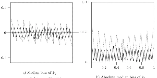
Bias, median-bias and their absolute values, M SE and M AD of the estimators are
exhibited in Fig. 2.1.4 - 2.1.7.
In Fig. 2.1.8 and Fig. 2.1.9, M SE and M AD of both estimators are compared
for samples of size n = 10 and n = 20 respectively. The figures demonstrate that
manipulations with empirical distribution function may introduce some asymmetry
in estimators as well as in their quality.
Fig. 2.1.4.
0.2
0.4
0.6
0.8
1
-0.1
0
0.1
...... ...... ... ...... ...... ... ...... ... .. .. .. .. .... .. .. .. .. .. .... .. ...... ...... ...... ... ...... ...... ... .. .. .. .. .. .. .... .. .. .. .. ...... ...... ...... ... ...... ...... ... .. .. .. .. .... .. .. .. .. .. .... .. .. .... ... ...... ... ...... ...... ...... .......... .. .. .. .. .. .. .... .. .. .. .. .. ... ... ...... ... ...... ...... .......... .... .. .... .. .... .. ... ...... ...... ...... ... .......... .. .. .... .. .. .. .. .. .... .. .. ... ...... ...... ...... ...... ... .......... .. .. .. .. .. .. .... .. .. .. .. .. ... ...... ... ...... ...... ...... .......... .. .. .... .. .. .. .. .. .... .. .. ... ...... ...... ...... ... ...... ...... ... .. .. .... .. .. .. .. .... .. .. .. .. .. ... ...... ... ...... ...... ... ...... ... ...... ...... ... ... ... ... ...... ...... ... ... ... ...... ...... ... ... ... ... ...... ......... ... ... ... ...... ...... ... ... ... ...... ...... ... ... ... ... ...... ... ... ... ...... ...... ......... ... ... ...... ...... ... ... ... ...... ... ...... ... ... ... ... ... ...... ... ... ... ... ... ...... ......... ... ... ... ...... ...... ... ... ... ...... ...... ... ... ... ... ...... ......... ... ... ... ...... ...... ... ... ... ... ...... ...... ... ... ... ...... ...... ... ... ... ... ...... ...... ... ... ... ... ... ... ... ... ... ... ... ... ... ... ... ... ... ... ... ... ... ... ... ... ... ... ... ... ... ... ... ... ... ... ... ... ... ... ... ... ... ... ... ... ... ... ... ... ...a) Median bias of ˆ
x
q
n = 10 dots, n = 20 solid
0.2
0.4
0.6
0.8
1
0
0.05
0.1
... ...... ... ...... ...... ... ...... ... ... ... ...... ........... .... .... .... .... .... .. .. .... .. .. .... .. ...... ... ...... ...... ... ...... ...... ... ...... ... .. .... .... .... .... .. .... .... .... ... ... ... ... ...... ... ... ... ... ...... ...... ... .... .... .... .... .... .. .... .... .... ... ...... ... ...... ... ... ... ...... .......... .... .... .... .... .. .... .... ...... ... ... ...... ... ... ... ...... ... ... ... .... .. .... .... .... .... .... ... ... ...... ... ... ... ... ... ... ... .... .. .. .. .. .. .... .. .. .. .. .. ...... ... ... ... ... ...... ... ... ........... .. .... .... .. .... .... .... .... .... ...... ...... ... ...... ... ...... ...... ... .. .... .... .... .... .... .... ... ... ...... ... ... ... ...... ...... ... ... .... .... .... .... .... .. .... .... .... ... ... ...... ... ... ... ...... ... ...... ...... ... .... .... .... .... .... .... .... .... .. .... ...... ... ... ... ...... ... ...... ...... ... ...... ... .. .... .... .... .... .... .... .... .. .... .... .... .... ...... ...... ......... ... ... ... ...... ...... ... ... ... ...... ... ...... ... ... ... ...... ...... ......... ... ... ... ... ...... ...... ... ... ... ...... ...... ... ... ... ... ... ...... ...... ... ... ... ... ... ... ...... ...... ...... ... ... ... ... ... ...... ...... ... ... ... ...... ...... ... ... ...... ......... ... ... ... ......... ... ... ...... ...... ... ... ... ... ... ...... ... ......... ... ... ... ...... ...... ... ... ... ... ...... ...... ......... ... ... ... ... ...... ...... ... ... ... ... ...... ......... ... ... ... ... ...... ...... ... ... ... ...... ...... ... ... ... ... ...... ...... ... ... ... ... ... . ...... ... ... ... ... ... ... ... ... ... ... ... ... ... ... ... ... ... ... ... ... ... ... ... ... ... ... ...b) Absolute median bias of ˆ
x
q
n = 10 dots, n = 20 solid
0.2
0.4
0.6
0.8
1
0
0.1
0.2
...... ........... .. .... ... .. ... ... ...... ............. ...... .......... .... ... ... ... ... ...... ...... ......... ...... ... ... ... ... ... ... ... ... ... ... ... ... ... ... ... ... ... ... ... ... ... ... ... ... ... ... ...c) M AD of ˆ
x
q
: n = 10 dots, n = 20 solid
Fig. 2.1.5.
0.2
0.4
0.6
0.8
1
-0.1
0
0.1
...... ...... ...... ...... ... ...... ........... .. .. .... .. .. .. .. .. .... .. ...... ...... ...... ...... ... ...... ... .. .. .. .. .. .... .. .. .. .. ... ...... ... ...... ...... ...... ... ... .. .. .. .... .. .. .. .. .... .. .. .... ...... ... ...... ...... ...... ... ... .... .. .. .. .. .... .. .. .. .. ...... ... ...... ... ...... ...... ... .. .... .. .... .. .... .. ... ...... ...... ...... ... .......... .. .... .. .. .. .. .... .. .. .. ... ... ...... ... ...... ...... ...... ... .. .. .. .. .... .. .. .. .. ...... ...... ...... ... ...... ...... .......... .. .... .. .. .. .. .... .. .. .. ... ... ...... ... ...... ...... ...... ... .. .. .. .. .... .. .. .. .. ...... ...... ...... ... ...... ...... ... ...... ...... ... ... ... ... ...... ......... ... ... ... ...... ...... ... ... ... ...... ...... ... ... ... ... ...... ......... ... ... ... ...... ......... ... ... ... ...... ......... ... ... ... ...... ...... ... ... ... ...... ...... ... ... ... ... ...... ... ...... ......... ... ... ... ...... ......... ... ... ... ...... ...... ... ... ... ...... ...... ... ... ... ...... ...... ... ... ... ... ...... ......... ... ... ... ...... ......... ... ... ... ...... ...... ... ... ... ...... ...... ... ... ... ... ...... ...... ... ... ... ... ... ... ... ... ... ... ... ... ... ... ... ... ... ... ... ... ... ... ... ... ... ... ... ... ... ... ... ... ... ... ... ... ... ... ... ... ... ... ... ... ... ... ... ... ...a) Bias of ˆ
x
q
: n = 10 dots, n = 20 solid
0.2
0.4
0.6
0.8
1
0
0.05
0.12
... ...... ... ...... ... ...... ...... ... ...... ...... ... ...... ... ...... ...... ... ... .. .. .. .... .. .. .. .. .. .. .. .. .. .... .. .. .. .. .. .. .. .. .. .. .... .. .. .. .... ...... ... ...... ...... ... ...... ...... ... ...... ... ... ... ...... ... ... .... .... .... .. .. .. .. .... .. .. .. .. .. .. .... .. .. .. .. .. .. ...... ...... ...... ... ...... ... ...... ...... ... ... ... .......... .... .... .... .... .... .. .. .. .... .. .. .. ... ... ... ... ...... ... ... ... ...... ... ... .......... .... .... .. .... .... .... .... .... .. ....... ...... ... ... ... ... ...... ... ... ... .... .... .... .... .... ... ... ... ... ... ... ... ... ... ... ... ... .. .. .. .. .... .. .. .. .. .. .... .. ... ... ...... ... ... ... ...... ... .. .... .... .... .... .... .... .... ... ... ...... ...... ... ...... ...... ... ... .. .... .. .... .... .... .... .... .... .... ...... ... ... ... ... ... ...... ... ...... ... ... ... ... .... .... .... .... .... .... .... .. .... .... .... .... ...... ... ... ... ...... ... ... ... ... ... ... ... ...... ... ... ........... .... .... .... .... .... .... .... .... .. .... .... .... .... .... .... ...... ... ... ... ... ... ... ... ... ... ... ... ... ... ... ... ... ... ... ...... ... .... .... .... .... .... .... .. .... .... .... .... .... .... .... .... .. .... .... .. ...... ...... ...... ...... ...... ... ... ... ... ... ... ... ... ... ... ... ... ... ... ...... ...... ...... ...... ... ... ... ... ... ... ... ... ... ...... ...... ...... ...... ... ... ... ... ... ... ... ... ...... ...... ...... ...... ... ... ... ... ... ... ... ... ... ...... ... ...... ......... ... ... ... ... ... ...... ...... ......... ... ... ... ... ...... ......... ... ... ... ... ... ... ... ... ... ...... ...... ...... ... ... ... ... ...... ......... ... ... ... ... ...... ......... ... ... ......... ... ...... ... ... ... ... ...... ... ... ... ... ...... ...... ... ... ... ...... ... ...... ... ... ... ... ... ...... ...... ... ... ... ... ... ... ... ...... ...... ... ... ... ... ... ...... ... ...... ...... ... ... ... ... ... ... ...... ... ...... ...... ... ... ... ... ... ...... ... ... ...... ... ... ... ... ... ... ... ...... ...... ... ... ...... ... ... ... ... ... ... ... ... ... ... .. ...... ... ... ... ... ... ... ... ... ... ... ... ... ... ... ... ... ... ... ... ... ... ... ... ... ... ... ...b) Absolute bias of ˆ
x
q
: n = 10 dots, n = 20 solid
0.2
0.4
0.6
0.8
1
0
0.1
0.2
...... ...... ........... .. .... .. .. .... .. ....... ... .... .......... .. ............... ......... ...... ... ... ... ... ...... ... ......... ... ... ......... ... ... ... ... ... ...... ......... ... ......... ...... ... ...... ... ... ... ... ... ... ... ... ... ... ... ... ... ... ... ... ... ... ... ... ... ... ... ... ... ... ...c) M SE of ˆ
x
q
: n = 10 dots, n = 20 solid
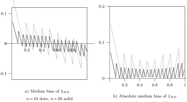
Fig. 2.1.6.
0.2
0.4
0.6
0.8
1
-0.1
0
0.1
... ...... ...... ... ...... ...... ...... ...... ... ...... ...... ... ...... ........... .... .. .. .. .. .. .... .. .. .. .. ... ...... ... ...... ...... ...... ... ... .. .. .. .... .. .. .. .. .. .... .. ...... ... ...... ...... ... ...... ...... ... .. .. .. .. .... .. .. .. .. .. .... .. .. ....... ...... ...... ...... ... ...... ... .... .. .. .. .. .. .... .. .. .. .. .. ...... ... ...... ...... ...... ... ...... .......... .. .. .. .. .. .... .. .. .. .. .. ...... ...... ...... ...... ... ...... ...... .... .... .. .. .. .. .. .... .. .. .. .. .. ... ...... ...... ...... ...... ... .......... .. .... .. .. .. .. .. .... .. .. .. ... ... ...... ...... ... ...... ...... ... ... .. .... .. .. .. .. .. .... .. .. .. ... ...... ...... ... ..... ...... ...... ...... ...... ... ... ... ... ...... ...... ... ... ... ... ...... ...... ... ... ... ...... ...... ... ... ... ... ...... ......... ... ... ... ...... ...... ... ... ... ... ...... ...... ... ... ... ...... ...... ... ... ... ... ...... ......... ... ... ... ...... ...... ......... ... ... ...... ...... ... ... ... ... ...... ......... ... ... ... ...... ...... ... ... ... ...... ...... ... ... ... ... ...... ......... ... ... ... ...... ...... ... ... ... ... ...... ...... ......... ... ... ... ...... ......... ... ... ... ...... .. ... ... ... ... ... ... ... ... ... ... ... ... ... ... ... ... ... ... ... ... ... ... ... ... ... ... ... ... ... ... ... ... ... ... ... ... ... ... ... ... ... ... ... ... ... ... ... ... ...a) Median bias of ˆ
x
HBn = 10 dots, n = 20 solid
0.2
0.4
0.6
0.8
1
0
0.1
0.2
...... ...... ...... ...... ...... ...... ...... ...... ...... ...... ...... ...... ... .... .. .. .. .... .. .. .. .... .. .... ...... ...... ...... ...... .......... .... .. .... .. .. .... .. .. ... ...... ...... ...... ...... ... .... .... .... .. ... ... ...... ...... ........... .... .... .... ... ...... ...... .......... .... .... .... ... ... ...... ...... ... .... .... .... .... .... ... ... ... ... ... ... ... ...... ... .... .... .... .... .... ... ... ... ... ... ... ... ... .......... .... .... .... .... .... .... .... ... ... ... ... ...... ... ... ... ... ... ... .... .... .... .... ... ...... ...... ...... ...... ......... ... ... ... ... ...... ...... ... ... ... ...... ... ... ...... ......... ... ...... ......... ...... ......... ... ... ......... ...... ... ...... ... ... ......... ... ......... ... ......... ...... ......... ... ... ...... ... ... ... ...... ... ... ... ...... ... ... ... ...... ... ... ... ...... ... ...... ... ... ... ...... ...... ... ... ...... ... ... ... ... ... ... ... ... ... ... ... ... ... ... ... ... ... ... ... ... ... ... ... ... ... ... ...b) Absolute median bias of ˆ
x
HBn = 10 dots, n = 20 solid
0.2
0.4
0.6
0.8
1
0
0.1
0.2
...... ...... ... ...... ... ...... ...... .... ... .. ... .. ... ...... ...... ... ... ... ... ... ... ... ... ... ... ... ... ... . ...... ...... ......... ... ... ...... ... ...... ...... ......... ...... ... ... ... ... ... ... ... ... ... ... ... ... ... ... ... ... ... ... ... ... ... ... ... ... ... ... ...c) M AD of ˆ
x
HB: n = 10 dots, n = 20 solid
Fig. 2.1.7.
0.2
0.4
0.6
0.8
1
-0.1
0
0.1
... ...... ... ...... ...... ...... ... ...... ...... ...... ... ...... ...... ........... .. .. .. .. .. .... .. .. .. .. .. ...... ...... ...... ... ...... ...... ... .. .. .... .. .. .. .. .... .. .. ...... ...... ...... ... ...... ...... ...... ... .. .. .... .. .. .. .. .... .. .. ... ...... ...... ... ...... ...... .......... .. .. .. .. .. .... .. .. .. .. ...... ... ...... ...... ... ...... ...... ........... .. .. .. .. .... .. .. .. .. .. ... ...... ...... ... ...... ...... ...... ... .. .. .. .. .. .... .. .. .. .. .... .. ....... ...... ...... ...... ... ...... ... .. .... .. .. .. .. .. .... .. .. .. ...... ...... ...... ...... ... ...... ...... .. .. .. .... .. .. .. .. .... .. .. .. .. .. .... ...... ...... ...... .... ...... ...... ...... ...... ... ... ... ...... ...... ......... ... ... ... ...... ...... ... ... ... ... ...... ...... ... ... ... ...... ...... ... ... ... ... ...... ......... ... ... ... ...... ......... ... ... ... ...... ...... ... ... ... ...... ...... ... ... ... ...... ...... ......... ... ... ... ...... ...... ... ... ... ...... ...... ... ... ... ... ... ...... ......... ... ... ... ...... ......... ... ... ... ...... ...... ... ... ... ...... ...... ... ... ... ... ...... ...... ... ... ... ... ...... ... ... ... ... ... ... ... ... ... ... ... ... ... ... ... ... ... ... ... ... ... ... ... ... ... ... ... ... ... ... ... ... ... ... ... ... ... ... ... ... ... ... ... ... ... ... ... ... ... ... ... ... ... ... ...a) Bias of ˆ
x
HB: n = 10 dots, n = 20 solid
0.2
0.4
0.6
0.8
1
0
0.1
0.2
...... ...... ...... ...... ...... ...... ...... ... ...... ...... ...... ...... ...... ...... ... .. .... .. .. .. .. .. .. .... .. .. .. .. ... ...... ...... ...... ...... ...... .......... .. .. .. .. .. .... .. .. .. .. ...... ... ...... ...... ...... ... ... .... .... .. .. .... ...... ... ...... ...... ........... .... ... ... ... ...... ...... ... .... .... .... .... ... ... ...... ... ...... ... .... .... .... .... .... .... ...... ... ... ... ...... ... ... ... ... .... .... .... .... .... .... .... ...... ... ... ... ... ... ... ... ... ... ... ... .... .... .... .... .... .... .... .... .... ... ... ... ... ... ... ... ... ... ... ... ... .... .... .... .... .... ... ...... ...... ...... ...... ......... ... ... ... ... ...... ...... ......... ... ... ... ...... ...... ......... ... ... ... ... ...... ......... ... ... ... ...... ... ... ... ... ...... ......... ... ...... ...... ... ... ... ... ...... ... ...... ... ... ......... ... ...... ... ... ...... ......... ... ... ...... ... ... ...... ...... ... ... ... ... ...... ......... ... ... ... ... ...... ... ... ... ... ... ... ... ...... ... ... ... ... ...... ... ...... ... ... ... ... ... ... ...... ... ... ...... ... ... ... ... ... ... ... ... ... ... ... ... ... ... ... ... ... ... ... ... ... ... ... ... ... ... ...b) Absolute bias of ˆ
x
HB: n = 10 dots, n = 20 solid
0.2
0.4
0.6
0.8
1
0
0.1
0.2
...... ... ...... ... ...... ...... ...... ........ ... .. .. .. .... .. ... ........ ... .... ... ......... ... ......... ...... ... ... ... ... ... ... ... ... ... ... ... ...... ... ...... ... ... .... ... . ...... ...... ...... ... ... ... ... ... ... ... ......... ...... ... ... ...... ... ... ...... ......... ...... ... ... ... ... ... ... ... ... ... ... ... ... ... ... ... ... ... ... ... ... ... ... ... ... ... ... ...c) M SE of ˆ
x
HB: n = 10 dots, n = 20 solid
0.2
0.4
0.6
0.8
1
0
0.1
0.2
...... ... ...... ...... ... .... ... .... ......... ...... ... ... ... ... ... . ...... ... ... ... ... ...... ......... ...... ... ... ...... ... ... ... ... ... ... ... ... ... ... ... ... ... ... ... ... ... ... ...n = 10
0.2
0.4
0.6
0.8
1
0
0.1
0.2
...... ... .......... ...... ...... ... ... .... ... ... ... ... ...... ...... ... ...... ... ... ... ... ... ... ... ... ... ... ... ... ... ... ... ... ... ... ...n = 20
Fig. 2.1.8. M AD of ˆ
x
HB- dots, ˆ
x
q
- solid
0.2
0.4
0.6
0.8
1
0
0.1
0.2
...... ...... ...... ...... ... ........ ... .... .. ... .......... .. .................. ............ ... ... ...... ... ... ... ... ... ... ...... ......... ... ... ... ... ......... ... ......... ... ...... ... ... ......... ... ...... ... ... ... ... ... ... ... ... ... ... ... ... ... ... ... ... ... ... ...n = 10
0.2
0.4
0.6
0.8
1
0
0.1
0.2
...... ...... ........... ......... ...... ...... ...... ... ... ... ... ... ... ......... ... ... ... ... ...... ... ...... ... ...... ... ... ... ... ... ... ... ... ... ... ... ... ... ... ... ... ... ... ...n = 20
Fig. 2.1.9. M SE of ˆ
x
HB- dots, ˆ
x
q
- solid
Though not fully satisfactory, we choose estimator ˆ
x
q
as a benchmark for assessing
other estimators below.
To the end we return to estimators which we rejected as ”defective” at the very
beginning of this Section. Fig. 2.1.10 exhibits absolute median-bias and M AD of
estimators x
(2)
q
= X
[nq]:n
, x
(3)
q
= X
[(n+1)q]:n
, x
(4)
q
= X
[(n+1)q]+1:n
, and the standard
0
0.2
0.4
0.6
0.8
1
0.1
0.2
... ... ... ...... .......... .... ...... ... ... ... ... ... ... ... ...... ... ... ... ...... ... ......... ... ... ... ... ...... ... ... ...... ...... ... ... .... ... ... ... ... ... ... ... ......... ... .... .... ... .... ... .......... .. ... ... ... ... .. ... ..... ....... .. .... .. ... . . . ... ... ......... . ... ... ... ...... ...... ... ... ......... ... ... ... ... ............ ... ... ... ...... ... ... ... ... ... ...... ... ...... ... ... ...... ... ... ... ... ... ... ... ... ... ... ... ... ... ... ... ... ... ... ...M AD
0
0.2
0.4
0.6
0.8
1
-0.2
-0.1
0
0.1
0.2
.... .... ........ ... .. .. ....... .... ........... .. .. ... ........ ... .... .. ... ........ ........... .... .. ... .... .... ............ .. .. ... .... ........... .. ... .... ... .. .... .. ... .... .... ............ .... .. ... ........ ....... .. .. .. ... . ... .. ..... . .. . ... .. .. ..... .. . . ... .. .. ... . . . ..... .. ...... . . ... .. ...... . .. . .. .. .. ...... .. . ... .. .. ..... .. . . ... .. .. ..... . . . ..... .. ... ... ... ... ... . ... ... ... ... ... . ...... ... ... ... ... . ... ... ... ... ... ... ... . ... ... ... ... ... . ... ... ...... ... ......... ... . ...... ... ... ... . ... ... ... ......... . ... ... ... ... ... ......... ... . ... ... ... ... ... ...... ...... ... ... ... ...... ...... ... ... ... ... ...... ...... ... ... ... ...... ...... ... ... ... ... ...... ......... ...... ......... ... ... ...... ...... ... ... ... ... ...... ...... ... ... ... ...... ...... ... ... ... ... ...... ...... ... ...... ... ... ... ... ... ... ... ... ... ... ... ... ... ... ... ... ... ... ... ... ...M edian Bias
Fig. 2.1.10. Mean Absolute Deviation and Median Bias of four estimators
...
ˆ
x
q
...X
[nq]:n
. . . .X
[(n+1)q]:n
... ... ... ... ... ... ....X
[(n+1)q]+1:n
We clearly see that from all those estimators only the estimator ˆ
x
q
deserves some
attention.
When estimating the median of an unknown distribution F
∈ F from a sample of
an even size 2n, estimator ˆ
x
q
is randomized: it chooses X
n:2n
or X
n+1:2n
with equal
probability 1/2; otherwise the estimator is not randomized. Let L
F
(T ) denote a loss
function of an estimator T when estimating the median of F . Then the risk of the
estimator T is E
F
L
F
(T ). For ˆ
x
0.5
from a sample of size 2n we have
E
F
(ˆ
x
0.5
) =
1
2
E
F
L(X
n:2n
) + E
F
L(X
n+1:2n
)
=
1
2
EL(U
n:2n
) + EL(U
n+1:2n
)
=
1
2
h Z
1
0
L(x)
(2n)!
(n−1)!n!
x
n−1
(1−x)
n
dx +
Z
1
0
L(x)
(2n)!
n!(n−1)!
x
n
(1−x)
n−1
dx
i
=
Z
1
0
(2n
− 1)!
(n − 1)!(n − 1)!
x
n−1
(1
− x)
n−1
dx
= EL(U
n:2n−1
) = E
F
L(X
n:2n−1
)
which means that the risk of the randomized estimator ˆ
x
0.5
from a sample of size
2n is is equal to the risk of the non-randomized estimator ˆ
x
0.5
from the sample of
size 2n
− 1. It follows that instead of randomization we may reject one observation
from the original sample: randomization for the median amounts to removing one
observation.
2.2. Local Smoothing
Given q, the local smoothing idea consists in constructing an estimator of the qth
quantile x
q
on the basis of two consecutive order statistics from a neighborhood
of X
[nq]+1:n
. Perhaps the best known example is the sample median which for n
being an even integer is defined as the arithmetic mean of two ”central” observations:
(X
n2
:n
+ X
n2+1:n
)/2. A possible rationale for the choice is as follows. According to
Definition (3)
F
n
(X
n2:n
) = lim
0<t→0
F
n
(X
n 2+1:n
− t) =
1
2
.
The left-continuous version of the empirical distribution function
F
n
0
(x) =
1
n
n
X
i=1
1
(−∞,x)
X
i
satisfies
lim
0<t
→0
F
0
n
(X
n2:n
+ t) = F
0
n
(X
n2+1:n
) =
1
2
so that there is no reason to choose X
n2
:n
instead of X
n2+1:n
or vice versa as an
es-timator for the median x
0.5
and to define the sample median depending on a choice
of the right- or a left-continuous version of the empirical distribution function.
Sta-tistical tradition suggests to take the mean of both. Another point of view on the
choice (X
n2
:n
+ X
n2+1:n
)/2 as an estimator of the median was presented in the
previ-ous section when discussing the cases of {nq} = 0.5 or q = 0.5. It appears that the
resulting estimator performs not very well in the very large statistical model F (see
Theorem 1 above).
More generally, a simple linear smoothing based on two consecutive order statistics
leads to the estimator
(7) ˆ
x
LS=
1 −(n +1)q +[(n +1)q]
X
[(n+1)q]:n
+
(n + 1)q −[(n + 1)q]
X
[(n+1)q]+1:n
which however is naturally defined for q ∈ [1/(n + 1), n/(n + 1)) only. A reason
for choice of (n + 1)q in (7) instead of nq as in (6) is that as a special case of (7)
we obtain the central value X
n2