A CASE STUDY IN SCHOOL
TRANSPORTATION LOGISTICS
Kazimierz Worwa*
*
Faculty of Cybernetics, Military Technical University, Warsaw, Poland, E-mail: kworwa@wat.edu.plAbstract In the paper, a school bus routing problem, its mathematical models and solution methods are investigated. The aim of the study is to search for school bus routing problem and its solution method and to apply them for a sample case study. The case study concerns the routing and scheduling of school buses in an exemplary, well-recognized school located in one of Polish community. The problem is to find a series of school bus routes that ensure the service is provided equitably to all eligible students. Because of the NP-hardness of the school bus routing problem, it is solved using some heuristic optimization method using real data from the considered exemplary school. The aim is to increase bus utilization and to reduce transportation times for students, while maintaining on-time delivery of students to the school. Although the problem under consideration is one of the earliest logistics problems solved using methods of operations research, remains valid and is the subject of research, as evidenced by numerous contemporary publications, presenting new methods for the formal specification and solution of the problem.
Paper type: Research Paper Published online: 31 January 2014 Vol. 4, No. 1, pp. 45-54
ISSN 2083-4942 (Print) ISSN 2083-4950 (Online)
© 2014 Poznan University of Technology. All rights reserved.
1. INTRODUCTION
Vehicle Routing Problem (VRP) is a typical logistic problem which has been widely studied on by many resarchers. It is also a classic example of the logistic problem solution of which is successfully supported by operational research methods, particularly mathematical modeling and optimization. VRP can be described as a problem of determining efficient routes for a fleet of vehicles in order to deliver or collect products from depots to a set of customers. Vehicle Routing Problem turns to be a relatively difficult problem when the number of inputs increases. This type of problem has been widely used in daily life so that trans-portation and distribution costs reflect as important cost elements into companies, enterprises, firms, schools etc. Human beings meet with VRP in different areas in daily life, for example various types of food and drink, clothing, heating material transportation, and garbage collection, postal service, personnel and student trans-portation. In this point of view, Vehicle Routing Problem separates into two main areas: human and freight transportation.
A typical application area of vehicle routing problems is School Bus Routing Problem (SBRP). In a large number of studies, SBRP is referred to as an important real world application of VRP. While a typical Vehicle Routing Problem mostly deals with the freight transportation, SBRP is related with people, e.g. students, transportation. Most school bus routing formulations focus on formulating extra constraints and objectives to take some student-related factors into account. Because of those reasons, SBRP problems are often more complicated than VRP. School Bus Routing Problem can be specified as follows: a group of spatially distributed students must be provided with public transportation from their resi-dencies to and from their schools. The problem is to find collection of some simple bus routes corresponding to buses selected from an available bus fleet that ensure the service is provided equitably to all eligible students. Student eligibility for school bus transportation is often determined by local school board according to accepted criteria, including distance between the place of residence and the school they attend. Additional restrictions are placed on the distance that students can walk from their homes to and from their stops. School bus routing problem has two separate routing issues: assigning students to bus stops and routing the buses to the bus stops. School bus routing is a version of the traveling salesman problem, commonly referred to the category of vehicle routing problems, either with or without time window constraints. In addition to the numerous studies that add-ressed the vehicle routing problem, various software methods have been developed that can utilized to minimize the operating cost. Three factors make school bus routing unique (Spasovic et al., 2001): efficiency (the total cost to run a school bus), effectiveness (how well the demand for service is satisfied) and equity (fairness of the school bus for each student). Although the School Bus Routing Problem is one of the earliest logistics problems solved using methods of
ope-rations research, remains valid and is the subject of research, as evidenced by numerous contemporary publications, presenting new methods for the formal spe-cification and solution of the problem.
The purpose of the considerations set out in the paper is to present a verbal and formal description of the School Bus Routing Problem (SBRP), to put forward some new suggestions for practical and effective solution and to apply them for a case study based on well-recognized school located in one of Polish community.
The remainder of the paper is organized as follows: Sections 2 and 3 present a general and mathematical descriptions of the SBRP, respectively. Section 4 presents a numerical example to illustrate the problem formulation and its solving method. Finally, Section 5 summarizes the presented considerations and provides concluding remarks.
2. GENERAL DESCRIPTION OF THE SBRP
Both, in the logistics and operations research literature, there are quite a few references to the School Bus Routing Problem as well as many different solution methods. SBRP has been constantly studied since the appearance of the first publi-cation on it (Newton and Thomas, 1969). However, a need for a general approach for SBRP remains as most studies on it have come about due to the appearance of real world problems which have specific assumptions and constraints. In a most common approaches to the SBRP it is decomposed into the following five main sub-problems:
1. bus stops selection,
2. assign eligible students to bus stops,
3. select buses from available bus fleet (the same or different types), 4. determine bus routes (assign bus stops to buses),
5. route scheduling.
Bus stop selection seeks to select a set of bus stops for students. For schools in rural surroundings, the students are assumed to be picked up at their homes. However, in urban areas, the students are assumed to walk to a bus stop from their homes and take a bus at the stop.
Bus stop selection is often omitted in the literature. Many studies assume that the locations of bus stops are given. Only a few papers considered bus stop selection, and most of them use heuristic algorithms. The heuristic solution approaches for bus stop selection are classified into the location-allocation-routing (LAR) strategy or the allocation-routing-location (ARL) strategy (Park & Kim, 2010).
After bus stops selection assigning eligible students to bus stops can be done. This allocation should be made taking into account the a number of restrictions regarding no more than a certain number of students can be assigned to the same bus stop; bus stops cannot be within a certain distance of each other; each student must be within a short walk of the bus stop and must not cross a major thoroughfare, etc.
Next step is to select buses from available bus fleet. Available bus fleet can consists of the same or different types of buses. In view of the need to minimize total transport cost the school boards are often interested in using minimum number of buses. In this aspect, important parameters are the bus capacity (number of seats), average speed, average fuel consumption, etc.
In bus route generation, the bus routes are constructed. The algorithms used in bus route generation can be classified into either the “route-first, cluster-second” approach or the “first, route-second” approach. The “route-first, cluster-second” approach builds a large route by a traveling salesman problem algorithm that considers all the stops, and partitions it into smaller routes considering the constraints. The “cluster-first, route-second” approach groups the students into clusters so that each cluster can be served as a route satisfying the constraints that exist. After the school routes are generated, improvement heuristics can be applied on the routes. There are a few of improvement heuristics and metaheuristic approaches proposed in literature (Park & Kim, 2010).
Route scheduling specifies the exact starting and ending time of each route and forms a chain of routes that can be executed successively by the same bus. In most studies, the starting and ending time of schools are constraints. However, there are a number of works that consider the times as decision variables and attempts to find the optimal starting and ending times to maximize the number of routes that can be served sequentially by the same bus and to reduce the number of buses used.
There are numerous and various constraints and requirements that can be considered when formulating the SBRP both in practice and in literature. The most comon are (Spada et al., 2005):
• vehicle capacity constraint: an upper bound on the number of students in a bus,
• maximum riding time: an upper bound on the travel time in a bus for each child,
• maximum walking distance: a student’s maximum allowable walking distance from his/her home to the bus stop,
• school time window: time window on the starting and ending arrival time of a bus at schools,
• upper bounds on the number of students at stops, • earliest pickup time for children,
• minimum number of children to create a route.
There are three objectives (measures) most commonly used for the SBRP (Spasovic at el., 2001): efficiency (the total cost to run a school bus), effectiveness (how well the demand for service is satisfied) and equity (fairness of the school bus for each student).
3.MATHEMATICAL FORMULATION OF THE SBRP
The mathematical models for SBRP are developed for various configurations. SBRP is usually formulated as mixed integer programming (MIP) or nonlinear mixed integer programming (NLMIP) models. However, most of them have not been used directly to solve the problems, and they are often not for the whole problem but for the SBRP parts (Park & Kim, 2010). In accordance with previous remarks the school bus routing has two main routing issues – assigning students to bus stops and routing the buses to the bus stops. In this section the SBRP consists of finding an optimizing collection of some simple bus routes corresponding to buses selected from an available bus fleet will be considered. The school bus routing problem can be presented conceptually as a linear cost minimization problem, in which the objective function is the total operating cost (Spasovic at el., 2001). The objective function can be minimized subject to a series constraints listed below:
1. each selected bus performs exactly one route, 2. each bus stop is allocated to only one bus, 3. every route must have at least one stop,
4. each route begins at school and arrives at school,
5. each selected bus stop can be visited by only one selected bus,
6. the number of students on each selected bus must not exceed the bus capacity, 7. accessible bus fleet has known number of the same buses,
8. the number of buses leaving the school must equal the number of buses re-turning to the school,
9. the travel time of each selected bus must not exceed the time duration allowed. Let I mean a set of allowed bus route numbers, I{1,2,3,...,i,...,I}. Let J mean a set of allowed bus stop numbers, J{1,2,3,...,j,...,J}, where the bus number 1 corresponds to the school. The set of bus stops, including the school, creates some bus stop network. Formally, a bus stop network can be defined as an undirected graph G=(J, E) with distances on the edges d: ER, where R+ is set of positive real numbers, and set J representing the bus stops is defined as follows: (i,j)E, if there is edge in G, connecting the vertices i, j, i.e. if after starting from the i-th stop as a next bus stop can be the j-th stop. It is convenient to represent the bus stop network G by means of a square matrix S[sij]JJ, where
otherwise. , if 0 (i,j) 1 sij E (1)
Additionally, we are given a bus capacity CN, where N is the set of natural numbers. In turn, in accordance with the constraints 1), 2) and 5) a bus number
I
i uniquely identifies the bus route. According to constraint 7) each bus iI
has the same capacity C. Let L mean a set of bus route numbers. In accordance with previous remarks we have LE, wherein LE if all buses were used to
transport students. We assume that it is also known a square distance matrix J J ij] d [
D , where element dijR is equal to the distance between i-th and j-th bus stops, if (i,j)E.
Let X[xijk]JJI mean a three-dimensional matrix, where element x ijk
is defined as follows otherwise. , bus of route to belongs and stops bus and if 0 k j i 1 s 1 xijk ij (2)
The matrix X will be called in further consideration as a school transport strategy. As a consequence of assumptions that have been determined and the definition (2) we have
otherwise. route bus by catered is stop bus if 0 , k i-th 1 x j ijk J (3)For the purpose of formulating of the exemplary SBRP we assume the following additional descriptions:
Tmax - maximum time available for the bus to pick up students on a route,
ni - number of students to be picked up at i-th bus stop,
K - operating cost for a bus (e.g. in € per bus-hour), V - average speed for a bus (e.g. in kilometers per hour).
The objective is to minimize total operating cost K(X) for a school transport strategy X that can be formulated as
) X ( T K ) X ( K i i
I , (4) where ) X (Ti is a time taken for bus k to pick up students on k-th bus route and drop students at school (node 1) can be roughly computed (excluding time to pick up students on k-th bus route and drop students at the school) as
) V / d x ( ) X ( T ij i j ijk i
J J . (5)On the base earlier assumptions and descriptions that were taken we can formulate the following formal optimization problem of the SBRP class:
minimize K(X) K T(X ) i i
I , (6)subject to the following set of constraints:
max i(X) T T , iI, (7) C ) n x ( i i j ijk
J J , kI, (8)1 x k j ijk
I J , iJ{1}, (9) 1 x k i ijk
I J , jJ{1}, (10) 1 x k j jk 1
I J , (11) 1 x k i k 1 i
I J , (12) 1 x j jk 1
J , kI, (13) 1 x j k 1 j
J , kI, (14)
J J j jik j ijk x x , kI, iI. (15)Constraints (7)-(16) have following interpretation:
• constraint (7) is to guaranty that the every bus do not travel over the time allowed,
• constraint (8) is to guaranty that every bus can take allowed number of students (capacity constraint),
• constraint (9) – (10) guaranty that every bus stop belongs to one bus route, • constraint (11) – (12) guaranty that there are at least one bus route,
• constraint (13) – (14) guaranty that every route is realized by exactly one bus, • constraint (15) is to guaranty the equality in the number of buses leaving
from and arriving to school.
4. NUMERICAL EXAMPLE
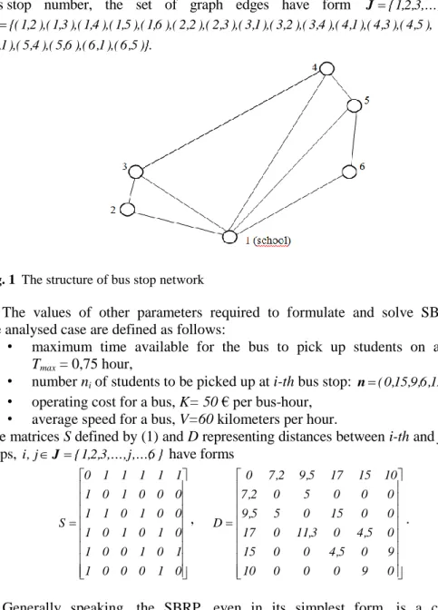
In this section an example of formulation and solving the School Bus Route Prob-lem will be presented. An example is based on the reality of one the Polish junior high school. The school must provide transportation of their students who use the designated bus stops in the area. The structure of bus stop network illustrates graph G, as shown in Figure 1.
The school under investigation has I=3 buses the same capacity C=30. Thus we have } 3 , 2 , 1 {
bus stop number, the set of graph edges have form J{1,2,3,...,j,...,6}, )}. 5 , 6 ( ), 1 , 6 ( ), 6 , 5 ( ), 4 , 5 ( ), 1 , 5 ( ), 5 , 4 ( ), 3 , 4 ( ), 1 , 4 ( ), 4 , 3 ( ), 2 , 3 ( ), 1 , 3 ( ), 3 , 2 ( ), 2 , 2 ( ), 6 , 1 ( ), 5 , 1 ( ), 4 , 1 ( ), 3 , 1 ( ), 2 , 1 {( E
Fig. 1 The structure of bus stop network
The values of other parameters required to formulate and solve SBRP for the analysed case are defined as follows:
• maximum time available for the bus to pick up students on a route, Tmax = 0,75 hour,
• number ni of students to be picked up at i-th bus stop: n(0,15,9,6,12,8),
• operating cost for a bus, K= 50 € per bus-hour, • average speed for a bus, V=60 kilometers per hour.
The matrices S defined by (1) and D representing distances between i-th and j-th bus stops, i,jJ{1,2,3,...,j,...,6} have forms
0 1 0 0 0 1 1 0 1 0 0 1 0 1 0 1 0 1 0 0 1 0 1 1 0 0 0 1 0 1 1 1 1 1 1 0 S , 0 9 0 0 0 10 9 0 5 , 4 0 0 15 0 5 , 4 0 3 , 11 0 17 0 0 15 0 5 5 , 9 0 0 0 5 0 2 , 7 10 15 17 5 , 9 2 , 7 0 D .
Generally speaking, the SBRP, even in its simplest form, is a complex and complicated. It can be proved thatthe combined problem of bus stop selection and bus route generation for a single school is an NP-hard problem. The bus route generation problem with vehicle capacity and maximum riding time constraints corresponds to a capacitated and distance constrained problem, which is known as an NP-hard problem (Bektas & Elmastas, 2007). Because of its complication only a few papers adopted exact approaches to solve the parts dealing on SBRP.
Due to its difficulty most studies prefer heuristic approaches rather than exact approaches (Park & Kim, 2010). Heuristics are defined as a set of rules that are being followed in solving complex pronlems. A few heuristic methods have been developed to provide the optimization for vehicle routing and scheduling problems that have time window constraints. One of the most known heuristic used to determine the solution of SBRP heuristic proposed by Clark and Wright, known as time saving heuristic (Clark & Wright, 1964).
Due to the small size of the analyzed example SBRP problem, finding its solution is relatively simple. Using any optimization package, e.g. Mathematica, gives the following optimal solution of the problem (6) - (15):
• number of bus routes, J=2,
• matrix X* [xijk]662, that maximizes objective function (4), for each of
the two buses, has the form
0 0 0 0 0 0 0 0 0 0 0 0 0 0 0 0 0 0 0 0 0 0 0 1 0 0 0 1 0 0 0 0 0 0 1 0 X1* , 0 0 0 0 0 1 1 0 0 0 0 0 0 1 0 0 0 0 0 0 0 0 0 0 0 0 0 0 0 0 0 0 1 0 0 0 X*2 ;
• optimal bus routes: 1) 1-2-3-1,
2) 1-4-5-6-1;
• optimal operating cost of bus routes: 36 , 0 ) X ( T1 * hour, T2(X*)0,68 hour, K(X*)50(0,360,68)52€. It is noteworthy that in the analyzed problem can be identified route 1-2-3-4-5-6-1 requiring of using only one bus, for which total operating cost is 42.5€. However, as can easily noted, this route should not be allowed to set routes, due to the failure constraints (7) and (8).
5. CONCLUSION
In this paper, the SBRP with regard to various aspects of the problem is described. Although the problems of the SBRP class are one of the earliest logistics problems solved using methods of operations research, they remain valid and are the subject of research, as evidenced by numerous contemporary publications. The paper presents an example of mathematical formulation and solving the problem of optimizing the school transportation system in one of the Polish junior high school. The small size of the problem made it possible to determine the exact solution.
REFERENCES
Bektas, T. & Elmastas, S., (2007), “Solving school bus routing problems through integer programming”. Journal of the Operational Research Society, Vol. 58, No. 12, pp. 1599–1604.
Bodin, L.D. & Berman, L., (1979), “Routing and scheduling of school buses by computer”. Transportation Science, Vol. 13, No. 2, pp. 113–129.
Clarke G. & Wright J.W., (1964) “Scheduling of Vehicles from a Central Depot to a Number of Delivery Points”, Operations Research, Vol.12, pp. 568-581.
Fisher, M.L., Jaikumar, R. & Van Wassenhove, L.N., (1986), “A multiplier adjust-ment method for the generalized assignadjust-ment problem”. Manageadjust-ment Scien-ce, Vol. 40, pp. 868–890.
Junhyuk P. & Byung-In K., (2010), “The school bus routing problem: A review”, Euro-pean Journal of Operational Research, 202, pp. 311–319.
Nagy, G. & Salhi, S., (2007), “Location-routing: issues, models and methods”. European Journal of Operational Research, Vol. 177, No. 2, pp. 649–672.
Newton, R.M. & Thomas, W.H., (1969), “Design of school bus routes by computer”. Socio-Economic Planning Sciences Vol. 3, No. 1, pp.75–85.
Park J. & Kim B.-I., (2010), “The school bus routing problem: A review”, European Journal of Operational Research, No. 202, pp. 311–319.
Simchi-Levi D. & Chen X., Bramel J., (2005), “The Logic of Logistics. Theory, Algorithms, and Applications for Logistics and Supply Chain Management”, Springer Science+Business Media, Inc.
Spada, M., Bierlaire, M. & Liebling, Th.M., (2005), “Decision-aiding methodology for the school bus routing and scheduling problem”. Transportation Science, Vol. 39, No. 3, pp. 477–490.
Spasovic L., S. Chien, C. Kelnhofer- Feeley, Y.Wang and Q. Hu (2001), “A Methodology for Evaluating of School Bus Routing - A Case Study of Riverdale, New Jersey”, Transportation Research Board Paper No. 01-2088.
BIOGRAPHICAL NOTES
Kazimierz Worwa is an Associate Professor at the Cybernetics Faculty of Military Technical University in Warsaw. He is deputy dean for education. His research interests include software reliability modelling, software testing methods and software efficiency. He is the author and co-author of many scientific publications. His paper appear in numerous journals, e.g. Control and Cybernetics or Polish Journal of Environmental Studies and proceedings of international conferences, eg. Depcos-Relcomex, Information Management or System, Modelling and Control.