Polarization vortices as a superposition of orthogonal
phase vortices
Władysław A. Woźniak*, Piotr Kurzynowski, Agnieszka Popiołek-Masajada
Department of Optics and Photonics, Faculty of Fundamental Problems of Technology, Wrocław University of Science and Technology, Wybrzeże Wyspiańskiego 27, 50-370 Wrocław, Poland
*Corresponding author. E-mail address: wladyslaw.wozniak@pwr.edu.pl ABSTRACT
The main idea of this paper is to explore the possibilities of expressing the polarization vortices as superposition of homogeneous orthogonally polarized waves with purely phase vortices. The relationships between the component phase vortices and the obtained polarization ones were investigated using different sets of polarization parameters. Presented numerical simulations and experiments led to the conclusion that the obtained kind of polarization vortices depends solely on the resultant charge of the component vortices (which is always the difference of the superposed vortices charge) and on the set of the used polarization parameters.
Keywords: optical vortices, optical singularities, polarization 1. Introduction
Optical point singularities play an important role in modern optics. They have become a subject of numerous investigations, thus forming a new chapter of optics: singular optics [1]. Singular optics deals with the topology of wavefronts. Starting with the well-known ray singularities (caustics) through the singularities of scalar fields researches come across more interesting cases: the polarization singularities of inhomogeneous vector fields. Polarization is one of light’s most significant features and describes the vector characteristics of the field. In addition to the phase’s point singularities there are also vector-point singularities (V-points). These kinds of singularities are characterized by the Poincaré-Hopf index which describes the vectors orientations in the surrounding planar vector field [2]. Even though the scalar field approach is limited to the simplest and most fundamental homogenous plane wave solutions of Maxwell’s vector wave equation, it still brings interesting results. Let Laguerre-Gaussian beams serve as an example: they can be classified both into scalar and vector types [3-7].
Different topological structures can exist in the generic polarized light field. For example, these structures can take three characteristic forms called star, lemon and moonstar around the points with pure circular polarization (C-point). Many researches were investigated the relations between these topological structures, their topology and statistics using only theoretical approach as well as describing experimental setups which allowed changes in these structures [8-19]. The relationships between the total topological charge of the optical vortices associated with linearly polarized orthogonal components were also investigated for various complex vector fields [12]. We believe that a different approach to this topic will also be interesting and will yield some new important conclusions.
Interferometry with phase singularities allows obtaining a new type of measurement standard with a stable and regular markers lattice [17]. This lattice can be generated in many different ways, for example, by way of nonlinear optical phenomena and a three homogenous plane-waves interference [20,21]. The new approaches to this generation techniques, using polarization elements (including spatial light modulators and anisotropic crystal elements), were also presented [22-25].
For example, the application of Wollaston prism in Mach-Zehnder interferometer [23] allowed obtaining a stable lattice of optical singularities identical to the one derived with three plane-waves interference. However, the use of the linear analyzer at the output of the proposed system revealed that the observed singularities are of phase character – all information about the polarization state of the interfering waves were lost. In our work [26] the polarization behavior of the obtained light field just prior to the analyzer was scrutinized and finally the conclusion was made that the type of phase singularities, achieved in the described system, depends on the polarization singularities and the kind of polarizer used at the end of the setup. Another conclusion was the idea that one can do the opposite: obtain polarization singularities from proper superposition of purely phase singularities, that is, with homogeneous polarization. This paper presents theoretical analysis as well as some experimental results of the superposition of orthogonally polarized light fields with phase vortices which leads to obtaining polarization vortices with different charges. Let us note that we limit our considerations to the superposition of plane wave fronts i.e. beams with a constant intensity distribution. Perhaps this differs from the current trendy considerations about Laguerre-Gaussian beams, but we think that such an approach can still give interesting results and besides, it is experimental realizable. Finally, the paper claims that polarization vortices can be expressed as superposition of homogeneous orthogonally polarized waves containing “pure” phase vortices.
2. Theoretical analysis
Let us remind some basic facts underlying our considerations. When two light fields described by the electric field intensity vectors E1
and E2
interfere with each other, the phase difference
between these two waves can be defined as:
1 2
argE E
(1)
where
denotes the scalar product of E1
and E2
. Quite trivial, but we often forget that this definition makes sense only if both of the light waves have the same polarization states at each point in the field. This is the only case where the resultant light field E can be defined as:
E e A
E i ˆ (2)
where A denotes the amplitude of the light and Eˆ stands for the unit vector representing the
same polarization state of both E1
and E2
field components. Now possible phase singularities in the light field can be found: when A0 the phase difference becomes undefined. What is more, if the difference at any point of the light field is undefined then the amplitude A (and
also the intensity) must be equal to 0. On the other hand, every light field (even “pure” phase field) can be described as a coherent superposition of orthogonally and homogeneously polarized light fields with well-defined difference . However, this distribution is not explicit and depends on
the choice of the light polarization state description (i.e. the base polarization states). It will be discussed later.
To describe the possible singularities in the light field with spatially inhomogeneous polarization state (polarization singularities) we require the vector approach. Let us assume that the resultant light field E can be described as:
1 2
1 2 1 ˆ1 2 ˆ2 cos ˆ1 sin ˆ2
i i
EE E E e E e I e e I e e (3)
where
I
denotes the light intensity of the resultant light field, ,1 denote the phases of both2components and eˆ1,eˆ2 are the basis’ orthogonal vectors of the component waves; stands for
the special quantity called the amplitude angle; tangent of is equal to the ratio of the components amplitudes. We have found this way of presenting amplitudes (and also intensities) dependencies more convenient as all other polarization quantities are denoted as “angles” (azimuth, ellipticity etc.). The relationships between the quantities , and the light polarization state
parameters depend on the used base eˆ1,eˆ2. With the imposing “simple” base of linear
polarization states Hˆ (“horizontal”) and Vˆ (“vertical”) we can notice that (where is a diagonal angle) and (where is a phase difference between x- and y- components of
electric field). This set is typical for Jones formalism [27]. With an alternative base of circular polarization states Rˆ (“right-handed”) and Lˆ (“left-handed”) we see that 290 (where
is an ellipticity angle) and 2 (where is an azimuth angle) – typical for Stokes formalism. Let us emphasize that the second option is used more often: the phase angle is
related to the azimuth angle of the light and indeterminacy of this quantity creates the most recognizable phase and polarization singularities – the C-points.
Finding potential singularities in the vector field represented by equation (3) is generally difficult; it is easier to look for zero places, suspected of being a singularity, for a scalar function. This function should take into account the superposition of E1
and E2
components, i.e. the overlap of at least the complex amplitudes of both field components.Such an useful function (as it turns out in a moment) may be, for example, the complex Stokes field [26]:
* 1 2 1 sin 2 2 i E fE E I e (4)
where 21 and * denotes the complex conjugation. This function loses information about
the vector character of the field but allows for a more comprehensive interpretation of its zero places. We will now call the phase angle as the imposing name “phase difference” seems
inadequate taking into account the limitation indication at the beginning of this paragraph. Let us note that in base of linear polarization states Hˆ and Vˆ we can rewrite function fE as:
sin 2 i E
f e (5a)
while using base of circular polarization states Rˆ and Lˆ:
2
cos 2 i E
f e . (5b)
The equation (3) and (in a more convenient way) equation (4) lead us to conditions that must be satisfied in order to obtain singularities in the light field. The amplitude term in Eq.(4) must be equal to 0 or one of the amplitudes in Eq.(3) must vanish. The condition I0 may indicate points where one can find singularities in a scalar field (homogeneous polarization) while the condition
0 2
sin can be a source of polarization singularities. Let us note that these conditions are
necessary for possible singularities but not sufficient – the factor determining the existence of singularity is the change of a parameter in the surroundings of a given point. Nevertheless, taking into account the described above relationships between polarization parameters , or , and , we can immediately see that possible polarization singularities can arise for
45
(undefined ) or for 090 (undefined ). In our paper we have limited our
observations only to the case of the superposition of two orthogonally but spatially homogeneously polarized light beams with phase singularities and all the above conclusions and statements may (but do not have to) relate to this special case.
3. Numerical simulations
We started our considerations on phase singularities superposition from numerical simulations. The both components were assumed to be homogeneously polarized light waves with orthogonal, linear polarizations. One or both of them may contain phase singularities – in fact, in our case only phase vortices with different topological charges will be taken into account. The phase vortices were created by introducing proper phase plates in one or both arms of our interferometric setup (see description in the next Section). Let us note that this way of vortices generation can change the relative width if Gaussian beams will be used, which will be observed later in the experiments. Taking into account all these simplifications the only parameters which will change in our numerical simulations are the chargesq1and q2 of both waves. Through simple and obvious
simulations visualizing formulas (3) and (4), we found that the obtained results depend only on the resultant charge q of calculated superposition. This resultant charge q is always the difference of the superposed vortices charges q1and q2 as the superposition of two waves in the
interferometric system means actually observing their differences. For obvious reasons, we did not present the results for q0 – superposition of two orthogonally polarized waves with vortices of the same charge. All parameters remained constant and no polarizing singularities appeared rendering the figures rather uninteresting (constant polarization parameters distributions). We investigated the superposition of the phase vortices with different topological charges and assumed that the clockwise vortices carry positive charges while anti-clockwise ones – negative. Without the decision as to which set of polarizing parameters will be used to present the results of our
experiments, we expressed the results of our numerical simulations in the form of and
parameters distributions. Figure 1 shows the results achieved for the superposition of the clockwise
1
1
q vortex with the homogeneous wave (q2 0) which means that the resultant charge q is
equal to 1. Let us note that in all the drawings here and in the next Section the same way of labeling the changes of the presented quantity was adopted: the smallest value is marked as blue, the highest as red through intermediate values indicated by the shades of green and yellow (note that the minimum and maximum values of each parameter differ). So, for example, for q1 1 and
0
2
q the minimum value of equals 0 (blue) while the maximum value 360 (red) while
parameter (part b) changes from 0 (blue) to 90 (red).
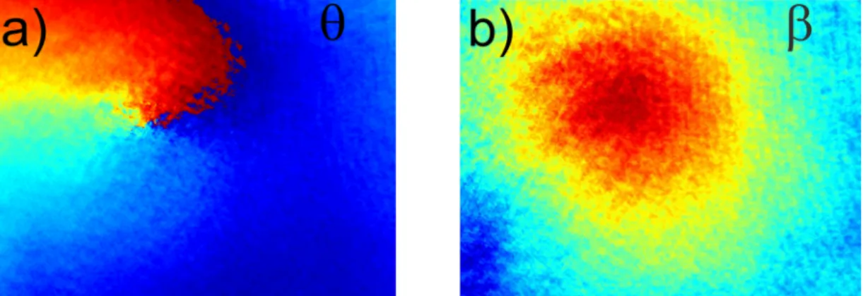
Fig. 1. Distributions of polarization parameters: a) and b) for the
superposition of the clockwise q1 1 vortex with the homogeneous wave (
0
2
q ).
Further numerical simulations have shown that identical graphs can be obtained for all of the situations in which the resultant charge q of both phase vortices is equal to 1. Hence, the results obtained by superposing for example the clockwise q1 2 vortex with the clockwise q2 1
vortex were exactly the same as for q1 1 and q2 0. What is more, the superposition of vortices with other resultant charges q will always yield the same shape of distribution of
parameter (part a) except for its the maximum value which now will be equal to q360 (red). And also all the figures presenting distribution of parameter (part b) will be exactly the same including the range of parameter variations.
It should be emphasized that using the system of and parameters we do not
predetermine in which base (linear or circular, see equations 5a and 5b) we will want to present the results of our experiments. Nevertheless, we can still show the distribution of polarization states in a “classical” way of ellipses and dashes. In this case, however, the distribution of polarization states around the vortex depends strongly on the resultant charge q of both vortices. Taking into account the limited scope of the subject of our paper, we will only show this distributions for the specific case of the resultant charge – here, for example, for q1and q2 (Figure 2).
Fig. 2. Representation of polarization distributions for the superposition of the homogeneous wave (q2 0) with a) the clockwise q1 1 vortex; b) the clockwise q12 vortex.
The characteristic vortex structures can be recognized in the centers of Fig.2a. The authors of this paper are convinced that by choosing phase vortices of different charges, one can generate any desired distribution of polarization singularities on high-order (or hybrid-order) Poincaré sphere [28,29] but the limited scope of the subject of this article and not the best quality of the conducted experiments (see nest Section) did not allow us to discuss it more widely.
No further charts are needed to draw general conclusions: superposing the phase vortices from two orthogonally polarized light fields results in the creation of polarization vortices in the resultant field. If we observe the phase angle , the vortex appears with the charge q equal to
the difference of the component charges (the Poincaré-Hopf index equal to +1). On the other hand, observation of the amplitude angle shows that this parameter has a regular maximum regardless of the charges of the phase vortices added.
4. Experimental verifications
To prove the correctness of our reasoning and presented simulations we made a superposition of two waves with phase vortices and orthogonal linear polarization states in an interferometric setup. The scheme of the experimental setup is presented in Fig. 3. The four beam splitters BS form a classical Mach-Zehnder interferometer. The plane, homogeneous wave of constant intensity (He-Ne laser, 0.633m) is incident on the polarizer P. The linear polarizer P with the azimuth
angle equal to 0 allows generating linearly polarized light in the both interferometer’s arms. The half-wave plate (HP) with the azimuth angle 45 placed in one of the arms rotates the polarization plane to orthogonal compared with the one in the other arm. Two spiral phase plates (SPP) generating phase vortices were placed in the both arms. The dimensions of the spiral phase plates were 1cm 1 cm and they introduced smooth 2q phase change for 0.633m wavelength where q is the vortex charge. The SPP with an appropriate q value was used as required. We used the Stokes Polarimeter (SP) described in [30] to determine the Stokes parameters of the light coming out of the setup which allowed calculating the parameters , and , .
Fig. 3. Scheme of the setup realizing the superposition of the plane waves with orthogonal polarization states and phase vortices.
The resultant light field’s polarization can be presented using both sets of polarization parameters ( , or , ) due to the fact that the type of polarization singularity may depend on the assumed set of parameters and the assumed base eˆ1,eˆ2 (Hˆ ,Vˆ or Rˆ,Lˆ). Taking into
account that both waves in our experiments are linearly polarized, the first set ( , ) was used as the proper one. However, also an experiment with circularly polarized component waves was carried out and in this case the second set ( , ) was used (see below).
The same way of labeling the quantity changes was used in all the drawings: the smallest value – blue, the highest value – red, intermediate values indicated by the shades of green and yellow. Let us note that the minimum and maximum values of each parameter are different: changes from
0 (blue) to 360 (red), changes from “almost 0” (blue) to “almost 90” (red). Taking into account that we use linear base of polarization states Hˆ and Vˆ we present the phase angle
as (part a) and the amplitude angle as (part b).
The following figures present the results of our experiments. Figure 4 shows the results of our system’s test: the superposition of two identical vortices in both interferometers arms with charge equal to 1. The resultant charge q (in the superimposed field) in this case is equal to 0 and all polarization parameters should have the same values in the whole measuring field. The numerical simulation for this special case was not discussed in the previous chapter as the simulated distributions were really uninteresting – now some artifacts caused by measurements inaccuracies distort the analysis of Fig. 3 but we have not observed any of the parameters discontinuities.
Fig. 4. Distributions of polarization parameters for superposition of two identical phase vortices with charge equal to 1 and the same signs (see description in the text) – experimental results.
Figures 5 and 6 show the experimental results of superposition of two different clockwise vortices with homogeneous wave q2 0. Figure 5 presents the results for clockwise q1 1
vortex (now the resultant charge q of interfering waves is equal to 1) while figure 6 presents the results for clockwise q12 vortex (resultant charge q is equal to 2). The resultant vortices with charges 1 and 2 are clearly visible in a) parts of both figures ( parameter), however, b) parts ( parameter) slightly differ. This is caused by the fact that Gaussian beam passing through SPP changes its width compared to the width of the homogeneous (q2 0) wave in the other arm of the interferometer.
Fig. 5. Distributions of polarization parameters for superposition of the clockwise q1 1
vortex with the homogeneously polarized wave (see description in the text) – experimental results.
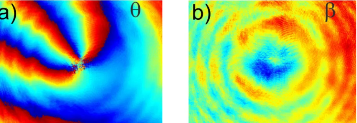
Fig. 6. Distributions of polarization parameters for superposition of the clockwise q12
vortex with the homogeneously polarized wave (see description in the text) – experimental results.
To investigate the influence of the beam widths mismatch mentioned above, we carried out two other experiments in which the resultant charge q of interfering waves was equal to 3. The charges of the component vortices, however, differed. Figure 7 presents the results of the interference of two beams with phase vortices with the same (clockwise) rotation and component topological charges q1 4 and q2 1. Figure 8 presents a bit different situation: the interference
of a clockwise q12 vortex with anti-clockwise q2 1 vortex. Note that the last case still
satisfies the principle of subtracting the component vortices charges: 2
1 3. If we disregard the inaccuracies of the setup adjustment (more complex that in the case of an interference with a homogeneous wave as both the vortices centers must be hit in the same point) the similarity and differences of the presented and distributions are clearly visible. The distributions are almost the same – broken symmetry and the changes in the direction of characteristic blue-red structure is caused by the different inclination of the interfering wavefronts. This is due to the possible inclination of plane-parallel plates which are SPP. The distribution for the second case (Fig. 8) is “flatter” than in the first case (Fig. 7) – the change of mutual curvatures of Gaussian beams made by SPP are smaller. The absolute values of SPP charges are similar, which results in comparable widths of the beams emerging SPP.Fig. 7. Distributions of polarization parameters for superposition of the clockwise 4
1
q vortex with the clockwise q2 1 vortex (see description in the text) – experimental
Fig. 8. Distributions of polarization parameters for superposition of the clockwise q12
vortex with the anti-clockwise q2 1 vortex (see description in the text) – experimental results.
Figure 9 shows the superposition of the clockwise q1 1 vortex with the anti-clockwise 1
2
q vortex resulting in the polarization singularity of the parameter with the resultant charge q2. This follows logically from the previous results but we decide to present it for two other reasons. Firstly, the same SPP plates (as for the absolute value of the vortices charges) generates identical widths of the beams, escaping the SPP plates and, finally, practically uniform distribution of the parameter (apart from a slight inclination due to the not eliminated slope of two interfering waves). The distribution of the parameter remains the same as shown in Fig. 6 (except for the rotation of the image).
Fig. 9. Distributions of polarization parameters for superposition of the clockwise q1 1
vortex with the anti-clockwise q2 1 vortex for linearly polarized light beams (see description in the text) – experimental results.
Secondly, using two quarter-wave plates with orthogonal first eigenwaves in both arms instead of the half-wave plate shown in Fig. 3 we ran an additional experiment with two circularly polarized light beams (right- and left-handed). Using the same SPP plates in both arms (the clockwise q1 1 vortex with the anti-clockwise q2 1 vortex) we obtained the similar results to the ones from linear polarizations. Figure 10 presents the results for circularly polarized components – the resultant charge q is still equal to 2 providing us with almost identical (as to character) distributions of both polarization parameters. Figures 9 and 10 are almost similar except of the parameters used (upper right corner). As it was mentioned at the beginning of Section 4, the experiment with circularly polarized component waves should use the second set of polarization parameters ( , ) – they are more suitable for Rˆ and Lˆ vectors used as a base. Let us note
that now parameter ranges from 0 (blue) to 180 (red) while ranges from 45 (blue) to +45 (red).
Fig. 10. Distributions of polarization parameters for superposition of the clockwise 1
1
q vortex with the anti-clockwise q2 1 vortex for circularly polarized light beams (see description in the text) – experimental results.
All the experimental results are affected by errors resulting from the insufficiently accurate adjustment of the system. In particular, one can see the parameters changes in each figure resulting from two facts: unavoidable inclination of both interfering beams and their astigmatisms (note the horizontal arcuate fringes on all distributions). This can cause all the straight lines from simulation become curves or even arcs. The main cause of all these inaccuracies lies, of course, in the design of the measuring system: the use of Mach-Zehnder configuration and spiral phase plates – this results in unavoidable changes in the curvature of Gaussian surfaces of both interfering beams. For these reasons, we gave up attempts to reconstruct the polarization state distributions in the form shown in Fig. 2 – the heterogeneities, especially visible in parts b) of all the above drawings, would make the resulting presentation illegible. Nevertheless, one can see a good agreement between the polarization parameter distributions obtained in our experiments and the simulations results. The polarization vortices with well-defined charges are visible in every a) parts of the figures (
parameter as or ) as well as continuous (as or ) parameter distributions in b) parts. 5. Conclusions
The main idea of this paper was to show that polarization vortices can be expressed as superposition of homogeneous orthogonally polarized waves containing “pure” phase vortices. We investigated the relationships between the component phase vortices and the obtained polarization singularities using different sets of polarization parameters depending on the used base. Our numerical simulations led us to the conclusion that the final effect depends only on the resultant charge q of the component vortices. In the case of interferometric superposition this resultant charge is always the difference of the superposed vortices charges q1and q2. Superposing the
phase vortices of two orthogonally polarized light fields results in the creation of polarization vortices in the resultant phase angle distribution. The choice of the polarization parameter,
however, which shows the character of the vortex, depends on the type of interfering waves. To prove the correctness of our reasoning we decided to conduct the experiments in Mach-Zehnder interferometer. Let us emphasize that our numerical simulations as well as experiments were made for plane parallel light waves with almost constant intensity – the influence of the Gaussian nature of interfering beams should be minimal. Although the experimental results are still affected by errors resulting from inaccurate adjustment of the system (the Gaussian curvature of both beams changed with the change of spiral phase plates), one can see good agreement between the polarization parameter distributions obtained in our experiments and in the simulations results. The polarization vortices with well-defined charges are visible in every a) part of the figures 3-9. Detailed analysis of the resulting polarization distributions, for example using a high-order or hybrid-order Poincaré sphere, would be possible in the theoretical part, but considerable experimental inaccuracies meant that we abandoned this idea. The more so because such classification goes beyond the main topic of this work.
References
1.M. Soskin, M. V. Vasnetov, “Singular Optics” in Progress in Optics, (Elsevier, 2001), Vol.
42, Chap.4.
2.V. I. Arnold, Geometrical Methods in the Theory of Ordinary Differential Equations, Vol. 250
of Grundlehren der Mathematischen Wissenschaften (Springer, 2012).
3.Q. Zhan, Cylindrical vector beams: from mathematical concepts to applications, Adv. Opt.
Photon. 1 (1) (2009) 1–57.
4.A. A. Tovar, Production and propagation of cylindrically polarized Laguerre–Gaussian laser
beams, J. Opt. Soc. Am. A 15 (10) (1998) 2705–2711.
5.E. J. Galvez, S. Khadka, W. H. Schubert, S. Nomoto, Poincaré-beam patterns produced by
non-separable superpositions of Laguerre-Gauss and polarization modes of light, Appl. Opt. 51 (15) (2012) 925-2934.
6.S. Vyas, Y. Kozawa, S. Sato, Polarization singularities in superposition of vector beams, Opt.
Express 21 (7) (2013) 8972-8986.
7.J. Wang, L. Wang, Y. Xin, M. Song, Polarization properties of superposed vector Laguerre–
Gaussian beams during propagation, J. Opt. Soc. Am. A 34 (2017) 1924–1933.
8.T. Ackemann, E. Kriege W. Lange, Phase singularities via nonlinear beam propagation in
sodium vapor, Opt. Comm. 155 (3-4) (1995) 339-346.
9.I. Freund, A. I. Mokhun, M. S. Soskin, O. V. Angelsky, I. I. Mokhun, Stokes singularity
relations, Opt. Lett. 27 (7) (2002) 545-547.
10. M. R. Dennis, Polarization singularities in paraxial vector fields: morphology and
statistics, Opt. Commun. 213 (4-6) (2002) 201-221.
11. O. V. Angelsky, A. I. Mokhun, I. I. Mokhun, M. S. Soskin, The relationship between
topological characteristics of component vortices and polarization singularities, Opt. Commun. 207 (1-6) (2002) 57-65.
12. I. Freund, Polarization singularities in optical lattices, Opt. Lett. 29 (8) (2004)
875-877.
13. K. Y. Bliokh, A. Niv, V. Kleiner, E. Hasman, Singular polarimetry: Evolution of
polarization singularities in electromagnetic waves propagating in a weakly anisotropic medium, Opt. Express 16 (2) (2008) 695-709.
14. M. M. Brundavanam, Y. Miyamoto, R. K. Singh, D. N. Naik, M. Takeda, K.
Nakagawa, Interferometer setup for the observation of polarization structure near the unfolding point of an optical vortex beam in a birefringent crystal, Opt. Express 20 (12) (2012) 13573-13581.
15. G. Milione, S. Evans, D. A. Nolan, R. R. Alfano, Higher Order Pancharatnam-Berry
Phase and the Angular Momentum of Light, Phys. Rev. Lett. 108 (19) (2012) 190401-1–190401-4. 16. M. V. Vasnetsov, M. S. Soskin, V. A. Pas’ko, Topological configurations of
cross-coupled polarization singularities in a space-variant vector field, Opt. Comm. 363 (2016) 181-187.
17. Sushanta Kumar Pal, Ruchi, P. Senthilkumaran, C-point and V-point singularity
lattice formation and index sign conversion methods, Opt. Comm. 393 (2017) 156-168.
18. Z. Liu, Y. Liu, Y. Ke, Y. Liu, W. Shu, H. Luo, S. Wen, Generation of arbitrary vector
vortex beams on hybrid-order Poincaré sphere, Photon. Res. 5 (1) (2017) 15-21.
19. Ruchi, Sushanta Kumar Pal, P. Senthilkumaran, Generation of V-point Polarization
Singularity Lattices, Opt. Express 25 (16) (2017) 19326-19331.
20. J. Masajada, B. Dubik, Optical vortex generation by three plane wave interference,
Opt. Commun. 198 (1-3) (2001) 21-27.
21. S. Eastwood, A. Bishop, T. Petersen, D. Paganin, M. Morgan, Phase measurements
using an optical vortex lattice produced with a three beam interferometer, Opt Express 20 (13) (2012) 13947-13957.
22. F. Flossman, U. T. Schwartz, M. Maier, Polarization singularities from unfolding an
optical vortex through a birefringent crystal, Phys. Rev. Lett. 95 (25) (2005) 253901-1– 253901-4. 23. P. Kurzynowski, W. A. Woźniak, E. Frączek, Optical vortices generation using the
24. Y. Liu, X. Ling, X. Yi, X. Zhou, H. Luo, S. Wen, Realization of polarization
evolution on higher-order Poincaré sphere with metasurface, App. Phys. Lett. 104 (19) (2014) 191110-1–191110-4.
25. C. Rosales-Guzmán, N. Bhebhe, A. Forbes, Simultaneous generation of multiple
vector beams on a single SLM, Opt. Express 25 (21) (2017) 25697-25706.
26. P. Kurzynowski, W. A. Woźniak, M. Borwińska, Regular lattices of polarization
singularities: their generation and properties, J. Opt. 12 (3) (2010) 035406.
27. R. Azzam, N. Bashara, Ellipsometry and polarized light, (Amsterdam: North-Holland
publishing company 1977).
28. M. J. Padget, J. Courtial, Poincaré sphere equivalent for light beams containing
orbital angular momentum, Opt. Lett. 24 (7) (1999) 430-432.
29. X. Yi, Y. Liu, X. Ling, X Zhou, Y. Ke, H. Luo, S. Wen, D. Fan, Hybrid-order
Poincaré sphere, Phys. Rev. A 91 (2) (2015) 023801-1–023801-6.
30. W. A. Woźniak, P. Kurzynowski, S. Drobczyński, Adjustment method of an imaging