Estimating the probability of optimal functioning for environment management systems and finding ways to improve their environmental reliability

S ł u p s k i e P r a c e G e o g r a f i c z n e 11 • 2014

Ivan Kirvel

Pomeranian University in Słupsk kirviel@yandex.ru

Piotr Shvedovskiy Aleksander Volchek

Briest National University, Bialorussia

ESTIMATING THE PROBABILITY OF OPTIMAL

FUNCTIONING FOR ENVIRONMENT MANAGEMENT

SYSTEMS AND FINDING WAYS TO IMPROVE THEIR

ENVIRONMENTAL RELIABILITY

OCENA PRAWDOPODOBIEŃSTWA OPTYMALNEGO

FUNKCJONOWANIA SYSTEMÓW I ZARZĄDZANIA

ŚRODOWISKIEM I WYZNACZENIE SPOSOBÓW

POPRAWY ICH NIEZAWODNOŚCI

Zarys treści: The optimal functioning of both natural and antropogenic systems is adequate-ly definable by parameters of ecological safety and sustainability. Practice shows that main factors determining the status and functioning of environmental management systems and environmental safety are design flaws, low construction quality and poor maintenance. This allows to improve ecological reliability by means of the initial reservation or to perform its gradual increase, implementing certain environmental rehabilitation measures. Performed analysis of Polesie water management systems had shown that optimal degree of prolonging the operation time by initial reservation should not exceed mi.r. = 1.38, while the optimal factor of the systems perfection should be not less than as. = 0.809, and factor of the allow-able investments increase into ecological reliability should not exceed mc. = 1.162. There-fore solution of providing the optimal ecological sustainability, reduncancy, and environ-mental management systems optimal functioning should be considered as a multi-criteria problem with the optimization on acceptable utility with maximum coherence, objective compromise, and preferability.

Key words:water resources, functioning, probability, environmental reliability, sustainability, analysis, optimization

Słowa kluczowe: zasoby wodne, funkcjonowanie, prawdopodobieństwo, zrównoważony rozwój, stabilność, analiza, optymalizacja

Introduction

As noted in Kirvel et al. (2013) the optimal functioning of natural, nature-antropogenized, and antropogenic systems is enough definable by the parameters of environmental safety and sustainability.

In this case, if the stability of the optimal functioning of the system determines its ability to maintain its structure and functional properties when exposed to exter-nal factors and to return close to its origiexter-nal state after exposure to factors that bring from balance, the probability of optimal functioning characterizes the probability that, during operation, the transition system from one state to another will not lead to a breach of its balance and its main parameters will not go over the critical limits. And, as shown in studies (Kirvel et al. 2013; Ivchenko, Martyshchenko 1998; Volchek et al. 2003), with a standard value of the required confidence probability γ = 0.9, lower confidence limit of the optimal functioning probability of the system (p) must be at least p = 0.986, at the prevailing indirect relationship between environ-mental components in range 0,697 ≤ R ≤ 0,732 – for direct interconnection, if the number of components (N) does not exceed 12.

In this case, regardless of the intended modalities and systems structure, their probability of optimal functioning can be described by the dependence (Shvedovskiy, Luksha 2001), given the reserve of environmental reliability level for all environmental components –

        ⋅ − ⋅ ⋅ −

_∑

_∑

− N , j > i N ij ij N = i i i η + q η + +( ) q q p = p 1 _1,2,... 1 0 1 ... 1 , (1) where p0 – the probability of the optimal functioning of the system if there is no

re-duction of environmental components reliability to a critical level; qi – the

probabil-ity of reaching the critical level of environmental reliabilprobabil-ity of any from the i-th component; ηi – weighting factor for the i-th component, which determines its

func-tional significance (redundancy); ηij, qij, … η1,2…N, q1,2…N – components weights and

probability of occurrence of double, triple, etc. superimposed processes of the envi-ronmental components reliability reduction; ηi = 1 - pi/p0; pi – the probability of

op-timal functioning of the system on reaching a critical level of environmental reliabil-ity of i-th component (Loginov et al. 2004).

Accordingly, at independence of the processes of achieving critical levels of en-vironmental reliability by the components, i.e. when p0 ≈ 1, we have

(

)

∏

− ⋅ N i= i i η q = p 1 1 . (2)

Analysis of survey materials of the environmental management systems state and functioning allows to note that main reasons of unsatisfactory performance and, con-sequently, low ecological reliability are design errors (18.9%), poor quality of build-ing (21.2%), poor maintenance (38.6%), and the set of all causes (21.3%). At the

same time 26% of them are already seen in the period of adaptation of systems, 29% – in the period of optimal functioning, and 45% – in the period of mass mani-festations of failure and the formation of a critical level of environmental safety.

Hence it follows that environmental reliability can be formed as by a primary reservation, so by its staged increase through the implementation of relevant envi-ronmental remediation. Let us consider this problem for the nature-antropogenized water management systems.

Results and discussion

Research carried out for the most common water management and agrolandscape Polesie systems with use of functional Bellman equations have revealed the estimat-ed terms of systems reconstruction to ensure maximal effect, which are: first recon-struction – 18, second – 33, third – 48, fourth – 67, fifth – 83 years.

However, in practice, the optimal reconstruction between lifespan of water sys-tems is 15 – 18 years at the maximum term of operation up to 30-33 years. For these time steps, we will optimize the environmental reliability and the probability of sys-tems optimal functioning.

Since the function of ecological reliability of any anthropogenic degree is defin-able by three regions (

3

1 = i

i

P ), four states of functioning ( 4

1 = j

j

S _{), ten factor variables of} risk (

S

₀₋₁₀

r

) and the set of real states of major groups of elements and components, then the following relationship can be used to optimize it:

(

)

[

]

∑

= − ⋅ + = t i t m opt com A +α C 0 1 0 θ 1 , (3) which takes into account both the initial capital investment, and the costs of provid-ing the required ecological reliability of the main group elements and the system as a whole. Here: А0 – one-time capital costs; θт – current annual cost of maintaining the

system performance at the required degree of environmental reliability;

(

)

[

]

1

1+α t − – factor of costs remoteness; α – normative coefficient of effectiveness; t – period of comparison.

Then, the economic effect of increasing the level of environmental reliability re-gardless of the method of its implementation can be determined by the following dependence

θ0´ = ky · En · t · (λ1 – λ2) – (C2 – C1), (4)

where λ1 – limit of costs increase of the system at increased calculation period and

improved ecological reliability by m times; λ2 – phasing factor of the

norma-tive factor of bringing costs; ky – specific capital investments; C1 and C2 – the

vari-ant-wise costs, respectively, of the elements main groups of the system, which are causing its environmental reliability as a whole.

It should be noted that the period of optimal environmental reliability is deter-mined by the period lof optimal functioning (Tк) (Braun et al. 1997; Heuvelink

1998; Kalinin et al. 2007).

Plots of the specific economic effect of increasing the calculation period and the level of environmental reliability of the system are shown in Fig. 1.

Эо m 1,5 1,0 0,5 0 1,5 3,0 4,5 6,0 7,5 lц эк bц эк 2,0 1,6 1,2 1,07 1,05 1,03 1 2 3 4 5 1а 2а 3а 4а

Fig. 1. Plots of the economic effect of improving the environmental reliability at (С1 - С2) = 0

(1a, 2a, 3a, 4a) and its economically allowable reduced costs increase at E = 0.08 (1, 2, 3, 4) and the reduced costs increase for providing the optimum environmental reliability at in-crease of the calculation period and the level (5): 1 – at T = 5 and T0 = 30; 2 – at T = 10 and

T0 = 30; 3 – at T = 15 and T0 = 30; 4 – at T = 30 and T0 = 30 years

Ryc. 1. Ryciny zależności efektu ekonomicznego od wzrostu bezpieczeństwa ekologicznego przy (С1 - С2) = 0 (1a, 2a, 3a, 4a) i ekonomicznie optymalnych wydatków przy E = 0,08 (1, 2,

3, 4) oraz zwiąkszenia trat na zabezpieczenia optymalizacji bezpieczeństwa ekologicznego, przy zwiększeniu okresu obliczanego i poziomu (5): 1 – dla T = 5 i T0 = 30; 2 – dla T = 10

i T0 = 30; 3 – dla T = 15 i T0 = 30; 4 – dla T = 30 i T0 = 30 lat

Analysis of the chart allows to note that the increase in calculation period and the level of environmental reliability is most appropriate to the period of formation of the critical level of environmental reliability (Тk) when optimizing the minimum

al-lowable level of environmental reliability and at the end of the initial (adaptation) period of operation – when optimizing the initial reservation.

Ө 0 eк ct eк ct

b

ℓ

Then the degree of economically reasonable increase in the cost of the system or basic groups of its elements is determined by the relation

0 0 2 1 ℓ С + L L = eк ct θ

, and the de-gree of increase of reduced costs to increase the calculation period or the level of environmental reliability ( eк

ct

b

) and the corresponding economic effect ( ' 0

θ

) by the relations –

b

eк

=

C

/ C

₀

ct and, where C0 – the costs of raising the calculation period

and the level of environmental reliability, given to the timing of environmental rehabil-itation works; L1 and L2 – are respectively the permissible costs for construction and

environmental reliability improvement of the main group of elements from the timing of T1 and T2 to the period Tc of the system operation (Rusin 1990; Jeffers 1981).

Accordingly, the allowable time frame to improve the calculation period and the level of environmental reliability at the construction stage determined by

2 1 M=L / L

Y indicator, and during the operational phase by –

k = k

_{д 1}

_⋅

Y

_М, where k1 –

the total cost of the basic version of the system.

Then the optimal degree of increase in the calculation period and the level of en-vironmental reliability of a group of elements of the system under construction is to be determined by the depen-dence (Truhaeva 1976)

(

)

1 1 2 1 _0.0953 1 1 . 1 ln ⋅ −         − − = T L L m c T opt , (5) where T1 – the duration of adaptation period of the system to form the ecological

environment state.

Accordingly, the period of optimal functioning (Тоpt) and the index of technical

perfection of the system (αk) are defined by –

(

)

(

)

(

)

(

)

(

)

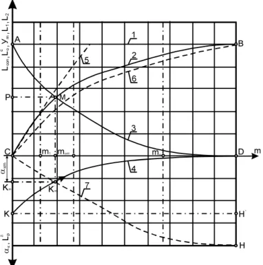
1 1 2 1 2 2 2 ln ln 1 1 1 1 1 1 1 оpt T_c T T T _c k L Т = + E L + + E T α = + E + E + E − − −       ⋅  _ _    _ − _   −    ₋ _{⋅ −}    _{  } . (6)

A graphical representation of these characteristics gives the generalized diagram of environmental safety and quality of systems (see Fig. 2).

Analysis of the main characteristics (1, 2, 3, 4) suggests the following.

At increase of the calculation period and the level of environmental reliability in the operation period the curve 2 approaches the straight line 1, with mкр·Т = Тс, i.e. at

equality of environmentally safe operation period of the whole system and major groups of elements (Т = Тс) permissible degree of increase in costs (mpr) reaches the

ceiling at the point B, where Ym = L1.

Improving the calculation period and the level of environmental reliability can also be achieved by increasing the perfection of main groups of elements, but the m times increase in the calculation period and the level of environmental reliability

А B P _M C m1 mопт mn D Km K_m' m K H H' α к , Lp δ α к m Lo c Lc o n , ,У m L1 L2 , , 1 2 5 6 3 4 7

Fig. 2. Generalized diagram of the level of environmental reliability and of technical per-fection of the system: 1 – L1 = f1(Т, Т_с); 2 – Y_m = f2(m, Т); 3 – L2 = f3(m, Т); 4 – αk = f4(m, Т);

5 – Lс = f5(m, Т); 6 – L = f

(

m,T

)

c 6

0 _{; 7 – L}b _=f

(

_m,T

)

р 7

Ryc. 2. Ugólniony diagram poziomu bezpieczeństwa ekologicznego i technicznego udosko-nalenia systemów: 1 – L1 = f1(Т, Т_с); 2 – Y_m = f2(m, Т); 3 – L2 = f3(m, Т); 4 – αk = f4(m, Т);

5 – Lс = f5(m, Т); 6 – L = f

(

m,T

)

c 6

0 _{; 7 – L}b _=f

₍

_m,T

₎

р 7

causes an increase in the level of technical perfection, which asymptotically ap-proaches its limiting value at D point (αк = 1). This means that the rate of cost of

en-vironmental protection and restoration activities in the operation of the system de-creases while the period of optimal functioning inde-creases. With a small optimal functioning calculation period the costs of raising the calculation period and the lev-el of environmental rlev-eliability are insignificant (at point А, L1 = L2).

The point P is characterized by indicators equality of costs for improving envi-ronmental reliability in the operation and providing the initial reservation of its cal-culation period.

M point of intersection of lines 2 and 3, characterized by an optimality (Ym = L2)

of functioning period with a given degree (level) of ecological reliability also de-fines the limits of the economic feasibility of improving performance by using the initial reservation (if the increase the calculation period of the main group of ele-ments is less than mопт times), and a phased implementation of conservation and

Accordingly, the definition of the achieved rate of the system perfection for any degree (the calculation period and level) can be done graphically designing mопт

point on the curve 4 (

_K

'_m) and then on the y-axis (

_K

'_m).

Analysis of additional dependencies (5, 6, 7) shows that the improvement of en-vironmental reliability determines concomitant increase in capital investments (Lc),

costs in conjugate area ( 0

c

L

) and reduces the cost of maintenance services (

L

b_р). These parameters are defined by

L

c

=

(

L

1

−

1

) (

/

L

2

−

1

)

; 1 2 0

/ L

L

=

L

c and L =Ym⋅

(

L2−1

) (

/ L2−1

)

b р . (7)

Drawing a vertical line at certain mi values, one can determine the values of the

above defined indicators and thereby more fully and accurately evaluate the effec-tiveness of measures to improve the calculation period and the level of environmen-tal safety.

Let’s analyze all these parameters and calculated dependence for the system, which is characterized by the following indicators: design life of the system – 30 years; period of operation of the system before the formation of the critical levels of environmental reliability at I variant T1=10 years and at II – Т2 =15 years; specific

capital investments C1 = $ 4.500 / ha and C2 = $ 6.000 / ha; normative to bring the

multi-temporal costs E = 0.1. Let’s plan to increase the calculation period of func-tioning with the calculated level of environmental reliability at I variant to 15, 20, 25 and 30 years and at II – 20, 25 and 30 years.

Being analyzed, the efficiency diagram of capital investments in the increase of ecological reliability of systems allows to note the following:

● optimal degree of the life functioning increasing by the initial reservation –

1.46 = mI opt and m =1.38; II opt

● permissible degree of the capital investments increase for the construction of an

object – _YmI₌1.186 _{and Y}II_=1.162;

m

● best perfection indicator of systems – αI=0.809

k and αII=0.829;

k

● the optimal duration of operation with confidence probability of optimal

func-tioning of γ = 0,9 and accordingly with the required environmental reliability, from the condition of minimizing the initial capital investment will be respec-tively _TI₌12.3

m years and TmII=16.9 years.

Conclusion

Water management and construction related to environmental management, envi-ronmental engineering in the field of water resources, formed today the variety of en-vironmental problems threatening not only the individual socio-economic interests of society, but also its whole vital activity through the deterioration of the environment.

Solving these problems requires both the development of methodologies for evaluating the probability of optimal operation of water systems and methodologies for evaluating changes in the level of environmental safety, stability, and reliability, especially at insufficient a priori information.

According to our research, the determining criterion of all the components caus-ing environmental sustainability, reliability, and optimum performance of systems is not only the value of specific capital investments, but also the knowledge of an op-timal timing of operation, the perfection index of a system, etc. Hence, this problem should be considered as a multicriteria problem with optimization at an affordable usefulness with the greatest consistency and target compromise. At the same time it should be based on the criteria of efficiency and preference.

References

Braun, P., Molnar T., Kleeberg H.B., 1997, The problem of scaling mgrid-related hydrologi-cal process modeling, Hydrologihydrologi-cal Processes, 11, p. 1049-1968

Jeferrs J., 1981, Introduction to system analysis and ecology application, Moscow

Heuvelink G.B.M., 1998, Uncertainty analysis in environmental modeling under a change of spatial scale, Nutrient Cycling in Agroecosystems, Vol. 50, p. 255-264

Ivchenko B.P., Martyshchenko L.A., 1998, Information technology, St. Petersburg

Kalinin M., Volchek A., Shvedovsky P., 2007, Hazardous Natural Disasters in Belarus, Nat-ural Disasters and Water Security: Risk Assessment, Emergency Response. and Environ-mental Management: abstract book, Yerevan, Armenia, 18-22 October 2007, International Geographical Union, Yerevan, p. 115-116

Kirvel I., Shvedovskaya D., Shvedowskii P., Volchek A., 2013, Ocena ekologiczna optymal-nego funkcjonowania systemów naturalnych i antropogenicznych, Słupskie Prace Geogra-ficzne, 10, p. 51-61

Loginov V.F., Volchek A.A., Shvedovskiy P.V., 2004, Application practice of statistics meth-ods at natural processes analysis and prediction, Brest

Rusin I.I., 1990, Ecologization of the economics: regional management methods, Moscow Shvedovskiy P.V., Luksha V.V., 2001, Mathematical modelling specifics of the development jumps

in ecology systems and processes, Vestnik Brestskogo universiteta, 2, 18, p. 29-31

Truhaeva R.I., 1976, The applied approach in researches of the decision making procedure, Moscow

Volchek А.А., Poita P.S, Shvedovskiy P.V., 2003, Mathematical methods in environmental engineering. Workbook for higher educational institutions, Minsk

Summary

The research is targeted at estimating the optimal functioning probability of natural, natu-ral-anthropogenic, and anthropogenic systems, and at determining ecological reliability and sustainability parameters for the hydroeconomic Polessie systems.

Analysis of the research results shows that solution of these problems is demanding their consideration as a multi-criteria ones with optimization at acceptable utility, with maximal coherence and objective compromise.