Assessment of potential transport of transport company for random demand for transport services

(1)

ASSESSMENT OF POTENTIAL TRANSPORT

OF TRANSPORT COMPANY FOR RANDOM DEMAND

FOR TRANSPORT SERVICES

Gustaw Konopacki*

* Institute of Information Systems Department of Cybernetics, Military University of Technology, Warsaw, Kaliskiego Str. 2, 00-908, Poland, E-mail: gkonopacki@wat.edu.pl

Abstract Will be considered transport company exploiting the uniform in the sense of destination, means of transport such as tankers, with a total transport potential equal to a loading units (e.g. tones). The company operates in the transport market, where demand for transport services is random. For-mulate the problem of satisfying the transport demand in full by transport company and shall be given the formulas to calculating the probability of such an event with the general assumptions about the demand for transport services. Practically useful formulas for estimating such a probability is given for the demand for transport services the described by normal stationary stochastic process. The re-sults are illustrated by an example of the calculation.

Paper type: Research Paper Published online: 30 October 2014 Vol. 4, No. 4, pp. 283-291

ISSN 2083-4942 (Print) ISSN 2083-4950 (Online)

(2)

1. INTRODUCTION

Important role of road transport in the economy should be seen in the fact that, among other modes, it stands out above all:

• mobility: you can get it anywhere where there are no rail, ship, etc.,

• high operability service, involving the availability of a relatively large number of means of transport,

• high high availability: getting lower car prices and getting better technical parameters,

• timeliness and punctuality performance of services.

Unfortunately. the major disadvantages of this type of transport are:

• dependent on climatic conditions, • not very eco-friendly,

• high rate of accidents,

• a relatively small volume of individual means of transport, • not very low maintenance costs of vehicle.

In practice, however, the advantages of road transport outweigh its disadvan-tages, what is the reason for its continued presence in the transport market.

One of the basic problems of the transport company managed is to provide its continued presence in the market of transport services, mainly by providing a appropriate potential transport for the anticipated demand for transport services.

The later in this chapter will be considered a problem of assessing the ability to satisfy a random demand for transport services by means of transport exploited in transport company at the expected time horizon.

2. DESCRIPTION OF THE PROBLEM

Will be considered transport company, in which are exploited vehicles (motor vehicles) for the same destiny (e.g. tanks), used to meet the demand for homogeneous transport services (e.g. carriage fuels). It is assumed that the cars do not have to be the same, i.e. not necessarily have the same design solution and the same payload. The transport potential transport company will constitute total capacity of all vehicles concerned. This potential will be denoted by a and treated as a constant, constant over time, the ability of a transport company to provide transport services at most this size. Whereas, transport demand generated by the transport market will be a time-varying random value. Therefore, you may experience the following two cases the lack of fit potentials transport companies to demand:

• demand for transport services may at some finite period of time can be less than the size of the potential transport,

• demand for transport services may at some finite period of time can be greater than the size of the potential transport.

(3)

These cases are temporary mismatches and take place only in finite time intervals whose lengths are dependent on the of the process characteristics of formation of the demand for transport services.

Next will be considered the second case, give rise to - it seems - more serious consequences for the transport company: inability to meet demand may lead to a reduction in the transport position of the company on the market of transport services, and even to his falling out of the market. In view of this it seems necessary to earlier understanding of the transport company as to either his possibilities to function on the transport market, in the case of having of the transport potential at the level of a. This knowledge may be useful to take pre-emptive action, such as the purchase of additional means of transport, or change of the profile provision of transport services.

3. FORMULATION AND SOLUTION OF THE PROBLEM

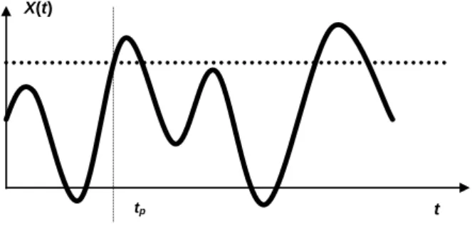
In the following discussion, it is assumed that random factors influencing the demand for transport services, while causing random changes its value, which will be described by a continuous-time stochastic process X(t). It is assumed that process X(t) is stationary, ergodic and differentiable in the mean-square sense (Gichman & Skorochod, 1968). Further issue will be considered for stochastic process X(t) is designated the probability of exceeded by this process a fixed value transport potential equal to a.In addition, the expected value of duration of such exceeded, i.e. the duration of exceeded by this process of fixed value transport potential equal to

a will be calculate. An exemplary implementation of stochastic process X(t) of

the change demand for transport services as a function of time is shown in Figure 1, in which tp indicates a moment of the exceeded value a through the process.

a

X(t)

t

tp

Fig. 1 An example of realization of the stochastic process X(t) describing the demand for transport services.

This problem determining of the probability distribution of residence time of a stochastic process X(t) over a defined threshold value a is computationally difficult. Fortunately, however, in practice, often enough to know the expected

(4)

value of the residence time of a stochastic process over a defined threshold value, which greatly facilitates the analytical solution.

The further considerations are true for any class of continuous-time stochastic processes, and final, practically useful computational formulas can be obtained relatively easily only for normal stochastic processes.

First will be considered the problem of determining the probability P(a,t) of the residence time of a stochastic process X(t) over a defined threshold value a. in the time interval [0,t].

Consider the probability that in the infinitesimal time interval dt, immediately following moment t, the process X(t) exceeds a threshold value a. This probability is presented in the following formula:

: P{X(t)aX(tdt)a} (1)

Given the assumption of continuity of the process X(t) and taking into account the rate of change of value of this process V(t), for arbitrarily small interval dt can be given the following formula:

(2)

Given the above equality in the expression (1) is obtained

(3) Let the f(x,v|t) will be density function of the two-dimensional distribution of the process X(t) and its speed V(t) at a moment t. Thus, the likelihood of (3) will be equal to:

(4)

where the limits of integration satisfy the following condition

(5)

After transformation of formula (5) with respect to that dt is arbitrarily small of interval time, is obtained

(6) Due to the fact that the probability of exceeded threshold a in the infinitesimal time interval dt is proportional to the length of this interval, you can use the density function p (a|t), denoting the probability exceeded threshold value a by the process

X(t) per unit time. Considering this assumption in the formula (3) is obtained:

(7)

From formulas (6) and (7) that:

(8)         0 a vdt a dxdv t) | v f(x, a} X(t) dt V(t) P{a 0 V(t) for a} X(t) dt V(t) P{a    dt V(t) X(t) dt) X(t   0 V(t) for a X(t) dt V(t) a          0 vdv t) | v f(a, a} X(t) dt V(t) P{a   0 vdv t) | v f(a, t) | p(a t) | p(a a} X(t) dt V(t) P{a   

(5)

Using the formula (8) can be calculated for each time interval of length T the expected value of residence time of the process X(t) over the threshold value a.

Let the above-mentioned time interval [0,T] is divided into n equal subintervals each of length dt, i.e. [tj, tj+dt], (j = 1,2, ..., n). Hence, the probability that the process X(t) exceeds the threshold value a in the time interval number j is equal to

(9) where h(x|t) is density function of the distribution of the process X(t) at a moment t.

If dt is sufficiently small that it will be possible to neglect cases multiple (at least double) crossing in each of these intervals the level a by the process X(t), the expected value of the residence time of the process above this level in the interval [0, T] is expressed by formula (see [Konopacki & Worwa, 2010]):

(10) In practical applications of interest is usually expected residence time of the process more than the threshold value is not in any period of time, but the expected duration of only one such clearance..Let  is a random variable representing the duration of a single crossing threshold value a by the process X(t). The expected value of this random variable is the quotient of the expected value E(Ta) and

the expected number of exceedances E(Na) of the threshold value a by the process X(t)

in the time interval of length T. Expected values of E(Na) and E() are expressed by

the following formulas (details in [Konopacki & Worwa, 2010, Pierievierziev, 1987]:

(11) (12) In the case of stationary process X(t), the density functions h(x| t) and f(x,v|t) no longer depend on the time and receive, respectively, the forms of h(x) and f(x,v). Thus, for stationary processes will apply the following formulas:

(13) (14) (15)     a dx ) t | h(x a} ) P{X(t_j _j

 

T  0 a a h(x|t)dxdt T E

 

T  





0 a a v f a,v t dvdt N E

 

      _  T 0 0 T 0 a dvdt t) | v f(a, v dxdt t) | h(x E

 

  a a T h(x)dx T E

 

   0 a T v f(a,v)dv N E      _  0 a dv v) f(a, v dx h(x) τ E

(6)

For the stationary process X (t) can be determined the expected number of ex-ceedances of threshold value a in the a unit of time, which is expressed by the fol-lowing formula:

(16)

To obtain a practically useful formulas necessary to know the density functions,

h(x) and f(x,v), which in the general case is difficult. Significantly simplifies the

situation in the case of a normal stationary stochastic process X(t). Unfortunately the describing processes the behavior of the demand for transport services under the action of random factors are not always stationary and additionally - normal. Thus, formulas obtained on the assumption stationarity and normality of the stochastic process X(t) have a definite cognitive value for the analysis of the considered problem, but the results obtained with their help should be considered only as approximate. Verification of these results is usually on the basis of statistics. Despite these reservations, however, take account of the stationarity and normality of the process X(t) is often the only option when is necessary a'priori to make a quantitative assessment of the problem, i.e., under conditions where there is not still the possibility of statistical studies the transport market.

Normal stationary stochastic process is clearly defined, when is known, mx and

Kx() - its expected value and correlation function. The density function of of the

process is as follows:

(17) where

(18) For stationary normal stochastic process its value and the rate of change of the value of the fixed point in time are independent random variables. Therefore, the density of a two-dimensional probability distribution f(x,v) in this case is equal to:

(19) where the variance 2

v

σ of process V(t) is equal to:

(20) and the expected value of this process is equal to zero due to the stationarity of the process X(t).

Taking into account the expression (19) in (16) we obtain:

 

     0 a a v f(a,v)dv T N E n      _   ₂ x 2 x x 2σ ) m (x exp π 2 σ 1 h(x) (0) K σ2 _x x              _   ₂ v 2 v 2 x 2 x x 2σ v exp π 2 σ 1 σ 2 ) m (x exp π 2 σ 1 v) f(x, 0 2 x 2 2 v d ) ( K d σ      









σ 2 m a exp n σ 2 m a exp πσ 2 σ n ₂ x 2 x 0 2 x 2 x x v a        _            _  

(7)

(21) where n0 is the expected number of exceedances through the process X(t) of its

expected value per unit of time.

Taking into account the expression (21) in (15) we obtain:

(22)

where the function (x) is the integral function of Laplace.

One of the most important practical questions in the management of the transport company is the problem of determining the likelihood that a time horizon of length T is not the demand for transport services, not once does not exceed a threshold value a, i.e. the transport potential of the transport company.. This is a problem difficult to solve by analytical methods, even in the case of normal stochastic processes. Help in the solution of this problem is when the expected number of exceedances of the threshold value in a certain period of time is small enough that the next exceedances of the threshold can be treated as independent random events. In this case, it can be assumed that the number of exceedances of the threshold value by the process is a random variable of Poisson distribution and problem of calculating the likelihood that in any time interval of length T there will be no exceeding of threshold value a by the considered process can be resolved in a satisfactory manner. Formulas (17-22) allow to calculate this likelihood for the stationary normal processes, which is equal to:

(23)

3. CONCLUSION

In solving practical problems, in general, there are the difficulties of establishing of analytical formula of correlation function as a function of the process X(t), which is necessary for the calculation of n0 value, which, in turn, is

essential to calculate the likelihood (23). In this case is most often accepted the upper estimate of this value that is equal to [Pierievierziev, 1987]:

(24) In the practical are often used estimate of likelihood of not exceeded of the threshold value for normal stationary stochastic process X(t) in the time interval of length T. There are:

lower estimate (25)

 





_























 

















_







σ

m

a

Φ

1 σ

2 m

a

exp

σ

π

E

x x 2 x 2 x v x



 

_{ }





σ 2 m a exp 0 K 0 K π 2 T exp T a, P ₂ x 2 x x " x 0                _       π 2 1 n₀                       ₂ x 2 x 0 x x min 0 0 σ 2 ) m (a exp T n σ m a Φ P T) (a, P

(8)

 upper estimate

(26) Estimating (25) can be use if T satisfies the following inequality:

(27)

If it is possible to observe the process X(t), value n0 can be estimated using

statistical methods without having to know the analytical form of the correlation function of the process.

The practical importance is the determination of the two values of transport potential:

 the upper limit, which is included in the above calculations performed,

 lower limit - limit of viability (e.g., economic) to provide transport services by transport company,

and determination of probabilities of exceeding each of them (the first up and the other down) through the process X(t). This is a problem more difficult than considered, but possible for a satisfactory solution.

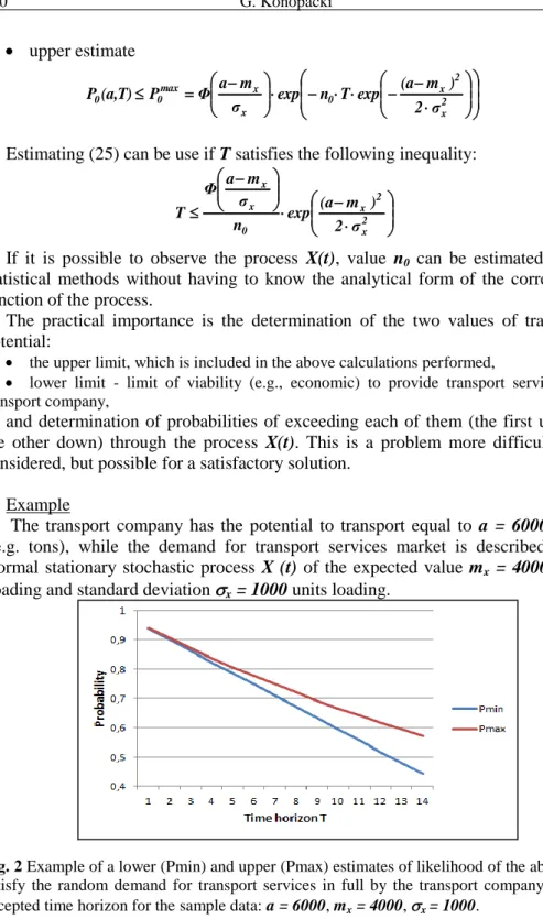
Example

The transport company has the potential to transport equal to a = 6000 units (e.g. tons), while the demand for transport services market is described by a normal stationary stochastic process X (t) of the expected value mx = 4000 units

loading and standard deviation x = 1000 units loading.

Fig. 2 Example of a lower (Pmin) and upper (Pmax) estimates of likelihood of the ability to satisfy the random demand for transport services in full by the transport company in the accepted time horizon for the sample data: a = 6000, mx = 4000, x = 1000.

                              ₂ x 2 x 0 x x max 0 0 σ 2 ) m (a exp T n exp σ m a Φ P T) (a, P                  ₂ x 2 x 0 x x σ 2 ) m (a exp n σ m a Φ T

(9)

Figure 2 shows the changes in the lower and upper estimates of the probability of not exceeding of the transport potential (the ability to satisfy the demand for transport services in full) by the demand on transport services as a function of time horizon T (e.g, months).

REFERENCES

Gichman I. I., & Skorochod A. W., (1968), Wstęp do teorii procesów stochastycznych,. PWN, Warszawa.

Feler W., (1996), Wstęp do rachunku prawdopodobieństwa, PWN, Warszawa.

Haggstrom O., (2001), Finite markov chains and algorithmic applications, Chalmers University of Technology.

Konopacki G., & Worwa K., (2010), „Problem eliminowania fałszywych alarmów w komputerowych systemach ochrony peryferyjnej”, Biuletyn Instytutu Systemów Informatycznych WAT w Warszawie, Nr 5/2010, s. 37-46.

Krawczyk S., (2001), Zarządzanie procesami logistycznymi, PWE, Warszawa. Lawler G. F., (1995), Introduction to Stochastic Processes, Chapman & Hall / CRC. Mitzenmacher M., & Upfal E., (2009), Metody probabilistyczne i obliczenia, WNT, Warszawa. Nowak M., (2007), „Strefy ochrony posesji”, dostępny w: www.budujemydom.pl.

Norris J. R., (1977), Markov Chains, Cambridge Series in Statistical and Probabilistic Mathematics.

Papoulis A., (1972), Prawdopodobieństwo, zmienne losowe i procesy stochastyczne, WNT, Warszawa.

Pierievierziev E.C. (1987), Słuczajnyje procesy v parametriczeskich modelach nadiożnosti. Naukovaja Dumka, Kijev.

Ross S.M. (1996), Stochastic processes. John Wiley & Sons, New York.. Sobczyk K., (1996), Stochastyczne równania różniczkowe, WNT, Warszawa.

BIOGRAPHICAL NOTES

Gustaw Z. Konopacki is an assistant professor at the Institute for Information Systems Department of Cybernetics of the Military University of Technology in Warsaw. He is also a an assistant professor at University of Warsaw. In 1990-1994 headed the Department of Computer Programming in the Department of Cybernetics MUT. Deals with the issues of modeling of safety and security facilities. Author of books on the design of information systems and co-author of four books of mathematical analysis and statistics. Author of more than eighty research publications. It deals mainly with the problems of mathematical modeling of processes.

(10)