Comparative study of photon
antibunching of non-stationary fields
A Miranowicz†
¶
, J Bajer‡
, H Matsueda†
, M R B Wahiddin§
andR Tana ´s
k
† Department of Information Science, Kochi University, 2-5-1 Akebono-cho, Kochi 780-8520, Japan
‡ Laboratory of Quantum Optics, Palack´y University, 772 07 Olomouc, Czech Republic § Institute of Mathematical Sciences, University of Malaya, 50603 Kuala Lumpur, Malaysia
k Nonlinear Optics Division, Institute of Physics, Adam Mickiewicz University, 61–614
Pozna´n, Poland
Received 22 December 1998
Abstract.Two standard criteria of the photon antibunching for non-stationary fields are compared. A new criterion, obtained by direct application of the Cauchy–Schwarz inequality, is proposed. All three definitions, based on the two-time correlation functions, are equivalent for stationary fields. However, the photon antibunching in the non-stationary regime is demonstrated to be not uniquely defined, since different criteria can lead to self-contradictory predictions. As an example, photon correlations of the signal mode in the parametric frequency converter are analysed analytically.
Keywords:Photon statistics, photon antibunching, frequency conversion
1. Introduction
Analysis of the photon-antibunching effect in nonlinear optical systems has been one of the hot topics of quantum optics for several decades. The theoretical and experimental search for the light exhibiting effect opposite to photon bunching has been triggered by the classic experiments of Hanbury Brown and Twiss [1]. Photon antibunching was first observed in the process of resonance fluorescence from an atom by Kimble et al [2] 20 years after the first photon-bunching demonstration [1]. Other successful generations of antibunched light in resonance fluorescence and in other nonlinear processes together with their detailed theoretical analyses have been summarized in a number of extensive reviews [3–6].
Although the experimental efforts have only focused on observing the photon-antibunching effects in stationary processes, there has also been some theoretical interest to analyse the photon antibunching of non-stationary fields. In particular, Kryszewski and Chrostowski [7] and Srinivasan and Udayabaskaran [8] analysed the photon antibunching of non-stationary fields of parametric frequency up-conversion with stochastic pumping. Singh [9] studied antibunching in resonance fluorescence in both stationary and transient non-stationary regimes. Dung et al [10] and Aliskenderov et al [11] analysed the non-stationary-field antibunching effects in the Jaynes–Cummings model, whereas Feng et al [12] studied the photon-antibunching effects in the model of light propagation through a nonlinear fibre with gain.
¶Permanent address: Nonlinear Optics Division, Institute of Physics, Adam Mickiewicz University, 61-614 Pozna´n, Poland.
The purpose of this paper is to show that the conventional descriptions of photon antibunching in non-stationary fields are by no means unique and might lead to self-contradictory interpretations of the results, i.e. a prediction of the photon antibunching according to one definition does not imply the photon antibunching occurs according to another. One can conclude that there are different photon-antibunching effects. To show these discrepancies explicitly, we analyse a model of parametric frequency conversion with initial signal and idler modes in Fock states. We have chosen this model to make our analytical comparison as simple as possible. Similarly, Zou and Mandel [13] analysed the simplest example of a plane, polarized electromagnetic field in the Fock state |{n}i to show the differences between the stationary-field photon antibunching and sub-Poissonian photon statistics. We are aware that the above models might not be useful for experimental verification.
This paper is organized as follows. In section 2, we give a short account of the most popular definitions of photon antibunching and we propose a new definition. In section 3, we briefly review the parametric frequency converter model for the purpose of our analysis of photon antibunching. In section 4, we show discrepancies between the definitions of photon antibunching for the non-stationary signal mode in the parametric frequency converter.
2. Definitions of photon antibunching
The most common definitions of photon bunching
and antibunching are based on the second-order two-time intensity correlation function (fourth-order amplitude
correlation function)
G(2)(t, t+ τ )= hT :ˆn(t)ˆn(t + τ) :i
= hˆa†(t )ˆa†(t+ τ )ˆa(t + τ)ˆa(t)i (1)
where ˆn(t) is the photon number operator, ˆa and ˆa† are,
respectively, annihilation and creation operators; the operator products are written in normal order (::) and in time order (T). The importance of the correlation function G(2)(t, t+ τ ) in
the analysis of photon antibunching comes from the direct relation of G(2)(t, t+τ ) to the joint detection probability [14]:
P2(t, t+ τ )1t 1τ= (αcS)21t 1τ G(2)(t, t+ τ ) (2)
of detecting two photons, one at time t and another at time
(t + τ ), by a photodetector of quantum efficiency α with a photocathode of area S. In (2), c denotes the velocity of light; the space coordinates are suppressed and only one photodetector is assumed.
The Cauchy–Schwarz inequality
[G(2)(t, t+ τ )]26 G(2)(t, t )G(2)(t+ τ, t + τ ) (3)
must be fulfilled for any classical field. Thus, the violation of inequality (3) can reflect the corpuscular nature of light and can serve as a criterion of antibunching effects.
Definition I. The photon antibunching (see, e.g., [3]) occurs if the two-time light intensity correlation function (1) increases from its initial value at τ= 0,
G(2)(t, t+ τ ) > G(2)(t, t ). (4)
This definition can be rewritten into the form (see, e.g., [4, 15])
1gI(t, t+ τ )≡ gI(2)(t, t+ τ )− g
(2)
I (t, t ) >0
(definition I) in terms of the degree of second-order temporal coherence
gI(2)(t, t+ τ )= G
(2)(t, t+ τ )
[G(1)(t )]2 (5)
which is the second-order correlation function G(2)(t, t+ τ )
normalized by the square of the mean photon number,
G(1)(t )= hn(t)i = hˆa†(t )ˆa(t)i. (6) The normalization is independent of τ . Inequalities for G(2)
and gI(2)describe the same effect assuming G(1)(t )6= 0.
Definition II. The photon antibunching (see, e.g., [2, 5]) takes place if the two-time normalized intensity correlation function (also called the degree of second-order coherence)
gII(2)(t, t+ τ )≡ λ(t, t + τ) + 1 ≡ G
(2)(t, t+ τ )
G(1)(t )G(1)(t+ τ ) (7)
increases from its initial value at τ = 0, i.e.,
1gII(t, t+ τ )≡ gII(2)(t, t+ τ )− g
(2)
II (t, t ) >0.
(definition II)
Definition III. Let us call the photon antibunching, the effect for which the two-time normalized intensity correlation function
gIII(2)(t, t+ τ )≡ G
(2)(t, t+ τ )
p
G(2)(t, t )G(2)(t+ τ, t + τ ) (8)
increases from its initial value at τ = 0, i.e.,
1gIII(t, t+ τ )≡ gIII(2)(t, t+ τ )− g
(2)
III (t, t ) >0.
(definition III) Photon antibunching can be defined in various ways by simply changing the normalization of G(2)(t, t+ τ ) by other τ-dependent functions. But probably the most natural way of defining photon antibunching is the direct application of the Cauchy–Schwarz inequality (3) as we propose in definition III. However, to the best of our knowledge, it has not yet been applied to analyse this effect even in the non-stationary regime (see, e.g., [7–12]).
According to the j th definition (j = I, II, III), photon bunching is said to exist if 1gj(t, t + τ ) < 0, and photon unbunching occurs if 1gj(t, t+ τ )= 0 for τ increasing from zero.
Definitions I–III can be rewritten in equivalent differential forms. Assuming that gj(t, t + τ ) is a well-behaved function of τ , the photon antibunching according to the j th definition occurs if the lowest-order (say n0)
non-vanishing derivative of gj(2)(t, t+τ ) [or 1gj(t, t+τ )] is greater than zero at τ= 0, i.e., n0> 1 exists such that
γj(t )≡ γ (n0) j (t )= ∂n0 ∂τn0g (2) j (t, t+ τ ) τ=0 >0 (9) and ∂n ∂τng (2) j (t, t+ τ ) τ=0 = 0 for n= 1, . . . , n0− 1. (10) For the purpose of our analysis, only the sign of the parameters γj(t ) = 0 is important. However, their values might be helpful in the analysis of the degree of antibunching. The field exhibits bunching if the lowest-order non-vanishing derivative, γj(t ), is negative. If the derivatives of all orders vanish, γj(t ) = 0, the field is said to be unbunched. In the following sections, we will use both parameters γj(t ) and correlation functions 1gj(t, t + τ ) to predict photon antibunching in a frequency conversion model for various initial fields.
Usually, the first derivatives γI,II(1)(t )are non-vanishing and in order to predict photon antibunching it is sufficient to determine their sign only e.g., parameter γI(1)(t )was used by Peˇrina [4], whereas γII(1)(t )was applied by Dung et al [10] and Aliskenderov et al [11]. Here, we give examples of the field evolution for which parameters γj(1)(t )vanish resulting in the analysis of the higher-order derivatives, in particular
2.1. Photon antibunching of stationary fields
Definitions I–III of photon antibunching are equivalent in stationary fields for which the condition
G(2)(t, t+ τ )= G(2)(τ ) (11)
is satisfied. Other equivalent definitions can be given in terms of the joint detection probability (2), as
P2(t, t+ τ ) > P2(t, t ) (12)
or with the help of the conditional probability
P2(t+ τ|t) ≡
P2(t, t+ τ )
P1(t )
(13) where P1(t )is the marginal probability.
Definitions I and II were originally proposed on the basis of the Cauchy–Schwarz inequality to describe antibunching of photons of stationary fields only. Inequality (3) implies that photon antibunching cannot occur for classical stationary fields, since they are described by a regular and non-negative
P-function.
2.2. Photon antibunching of non-stationary fields The question arises how to describe photon bunching and an-tibunching for non-stationary fields? Or, explicitly, which of definitions I–III is the closest to the original meaning of ton antibunching—the effect reflecting the tendency of pho-tons to preferentially distribute themselves separately rather than in bunches, when the intensity of light is not stabilized? We show that the predictions of photon antibunching according to definitions I–III might be essentially different for non-stationary fields, though they coincide in stationary
fields. Differences between various approaches to
antibunching result from the normalization functions of
G(2)(t, t + τ ), which for definition I is independent of τ ,
whereas for definitions II and III is τ -dependent, but in two non-equivalent ways of non-stationary fields.
There have been some theoretical investigations of the antibunching effect occurring not only in stationary regime. In fact, both definitions I and II of photon antibunching have been applied to analyse non-stationary fields. For applications of definition II see, e.g., [7, 8, 10, 11], and for definition I see, e.g., [9, 12]. To the best of our knowledge, definition III has not been used yet in the analysis of the antibunching effect. However, for non-stationary fields, only definition III implies violation of the Cauchy–Schwarz inequality (3).
3. Model for testing antibunching
We analyse different kinds of bunching and antibunching of photons in a process of parametric frequency conversion. The model can be described by the interaction Hamiltonian [16]:
ˆ
Hint= ¯hκ ˆaaˆab†exp(i1ωt) + h.c. (14) where 1ω = ω + ωb− ωa, and ˆaa,b are the annihilation operators for the signal (with subscript a) and idler (subscript
b) modes; κ is the real coupling constant. For simplicity, we only analyse the resonance case, 1ω= 0.
There are simple trigonometric solutions for the signal and idler modes in the interaction picture [16]:
ˆaa(t )= cos(κt) ˆaa− i sin(κt)ˆab ˆab(t )= cos(κt) ˆab− i sin(κt)ˆaa
(15) whereˆaa,b≡ ˆaa,b(0). All expressions for the second mode are given by those for the first mode albeit with interchanged subscripts. The constant of motion is
hna(t )i + hnb(t )i = hna(0)i + hnb(0)i = const. (16) We have chosen a two-mode model to analyse antibunching in the signal mode only. The idler mode gives us the possibility of manipulating the photon-number statistics of the signal mode.
4. Different predictions of photon antibunching Let us analyse the parametric frequency conversion of the signal and idler modes initially in Fock states with photon numbers Naand Nb, respectively. By applying the solution (15) to (1) and (6), we find the two-time intensity correlation function for the signal mode
G(2)(t1, t2)= Na(Na− 1) cos2(κt1)cos2(κt2)
+NaNbsin2[κ(t1+ t2)]
+Nb(Nb− 1) sin2(κt1)sin2(κt2) (17)
and the signal mean photon number
hna(t )i = Nacos2(κt )+ Nbsin2(κt ). (18) For brevity, hereafter we present correlation functions for the signal mode only. Therefore, we can consequently omit subscript a in correlation functions
G(2)(t1, t2)≡ G(a2)(t1, t2),
gj(2)≡ gj,a(2), 1gj ≡ 1gj,a
(19) for j = I, II, III. Due to the symmetry of the solutions (15), one can deduce the explicit expressions for the idler mode by simply interchanging the subscripts.
Exact analytical solutions for the normalized correlation functions gj(2)(t, t+ τ ) (j = I, II, III) defined, respectively, by (5), (7) and (8), are obtained from (17) and (18) in a straightforward way. Then the exact solutions can be represented graphically for better comparison (see, e.g., figure 4). We would like to give analytical self-evident comparison of different definitions. Since, photon antibunching is defined in the short-time separation limit, we expand gj(2)(t, t+ τ ), or alternatively 1gj(t, t+ τ ), in Taylor series in τ . We find 1gI(t, t+ τ )= sin(2κt) 2hna(t )i2 {−Na(Na− 1) cos2(κt ) +2NaNbcos(2κt ) + Nb(Nb− 1) sin2(κt )}(κτ) +O(τ2) (20) 1gII(t, t+ τ )= NaNb sin(2κt ) hna(t )i3 {(Na+ 1) cos2(κt ) −(Nb+ 1) sin2(κt )} (κτ) +O(τ2) (21) 1gIII(t, t+ τ )= − NaNb 2[G(a2)(t, t )]2 {2Na(Na− 1) cos4(κt ) −(NaNb+ Na+ Nb− 1) sin2(2κt) +2Nb(Nb− 1) sin4(κt )}(κτ)2+O(τ3). (22)
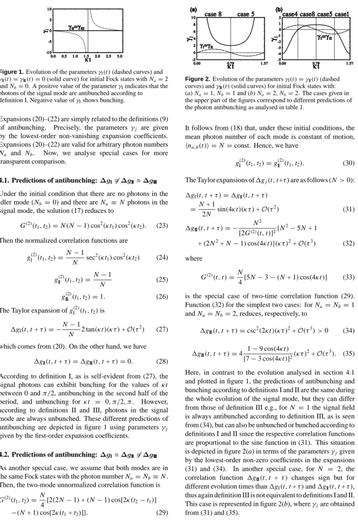
Figure 1.Evolution of the parameters γI(t )(dashed curves) and
γII(t )= γIII(t )= 0 (solid curve) for initial Fock states with Na= 2
and Nb= 0. A positive value of the parameter γIindicates that the
photons of the signal mode are antibunched according to definition I. Negative value of γIshows bunching.
Expansions (20)–(22) are simply related to the definitions (9) of antibunching. Precisely, the parameters γj are given by the lowest-order non-vanishing expansion coefficients. Expansions (20)–(22) are valid for arbitrary photon numbers
Na and Nb. Now, we analyse special cases for more transparent comparison.
4.1. Predictions of antibunching:∆gI6=∆gII=∆gIII
Under the initial condition that there are no photons in the idler mode (Nb = 0) and there are Na ≡ N photons in the signal mode, the solution (17) reduces to
G(2)(t1, t2)= N(N − 1) cos2(κt1)cos2(κt2). (23)
Then the normalized correlation functions are
gI(2)(t1, t2)= N− 1 N sec 2(κt 1)cos2(κt2) (24) gII(2)(t1, t2)= N− 1 N (25) g(III2)(t1, t2)= 1. (26)
The Taylor expansion of gI(2)(t1, t2)is
1gI(t, t+ τ )= −
N− 1
N 2 tan(κt)(κτ ) +O(τ
2) (27)
which comes from (20). On the other hand, we have
1gII(t, t+ τ )= 1gIII(t, t+ τ )= 0. (28)
According to definition I, as is self-evident from (27), the signal photons can exhibit bunching for the values of κt between 0 and π/2, antibunching in the second half of the period, and unbunching for κt = 0, π/2, π. However, according to definitions II and III, photons in the signal mode are always unbunched. These different predictions of antibunching are depicted in figure 1 using parameters γj given by the first-order expansion coefficients.
4.2. Predictions of antibunching:∆gI=∆gII6=∆gIII
As another special case, we assume that both modes are in the same Fock states with the photon number Na= Nb≡ N. Then, the two-mode unnormalized correlation function is
G(2)(t1, t2)=
N
4{2(2N − 1) + (N − 1) cos[2κ(t2− t1)]
−(N + 1) cos[2κ(t1+ t2)]}. (29)
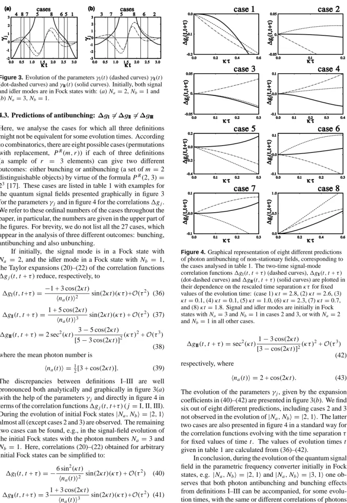
Figure 2.Evolution of the parameters γI(t )= γII(t )(dashed
curves) and γIII(t )(solid curves) for initial Fock states with:
(a) Na= 1, Nb= 1 and (b) Na= 2, Nb= 2. The cases given in
the upper part of the figures correspond to different predictions of the photon antibunching as analysed in table 1.
It follows from (18) that, under these initial conditions, the mean photon number of each mode is constant of motion,
hna,b(t )i = N = const. Hence, we have
g(I2)(t1, t2)= g(II2)(t1, t2). (30)
The Taylor expansions of 1gj(t, t+τ ) are as follows (N > 0):
1gI(t, t+ τ )= 1gII(t, t+ τ ) = N+ 1 2N sin(4κt)(κτ ) +O(τ 2) (31) 1gIII(t, t+ τ )= − N2 [2G(2)(t, t )]2{N 2− 5N + 1 + (2N2+ N− 1) cos(4κt)}(κτ)2+O(τ3) (32) where G(2)(t, t )=N 4[5N− 3 − (N + 1) cos(4κt)] (33) is the special case of two-time correlation function (29). Function (32) for the simplest two cases: for Na = Nb = 1 and Na= Nb= 2, reduces, respectively, to
1gIII(t, t+ τ )= csc2(2κt )(κτ )2+O(τ3) >0 (34)
1gIII(t, t+ τ )= 4
1− 9 cos(4κt) [7− 3 cos(4κt)]2(κτ )
2+O(τ3). (35)
Here, in contrast to the evolution analysed in section 4.1 and plotted in figure 1, the predictions of antibunching and bunching according to definitions I and II are the same during the whole evolution of the signal mode, but they can differ from those of definition III e.g., for N = 1 the signal field is always antibunched according to definition III, as is seen from (34), but can also be unbunched or bunched according to definitions I and II since the respective correlation functions are proportional to the sine function in (31). This situation is depicted in figure 2(a) in terms of the parameters γjgiven by the lowest-order non-zero coefficients in the expansions (31) and (34). In another special case, for N = 2, the correlation function 1gIII(t, t + τ ) changes sign but for
different evolution times than 1gI(t, t+ τ ) and 1gII(t, t+ τ ),
thus again definition III is not equivalent to definitions I and II. This case is represented in figure 2(b), where γjare obtained from (31) and (35).
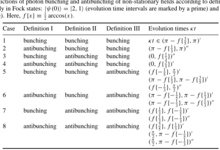
Figure 3.Evolution of the parameters γI(t )(dashed curves) γII(t )
(dot-dashed curves) and γIII(t )(solid curves). Initially, both signal
and idler modes are in Fock states with: (a) Na= 2, Nb= 1 and
(b) Na= 3, Nb= 1.
4.3. Predictions of antibunching:∆gI6=∆gII6=∆gIII
Here, we analyse the cases for which all three definitions might not be equivalent for some evolution times. According to combinatorics, there are eight possible cases (permutations with replacement, PR(m, r)) if each of three definitions (a sample of r = 3 elements) can give two different outcomes: either bunching or antibunching (a set of m= 2 distinguishable objects) by virtue of the formula PR(2, 3)= 23[17]. These cases are listed in table 1 with examples for the quantum signal fields presented graphically in figure 3 for the parameters γjand in figure 4 for the correlations 1gj. We refer to these ordinal numbers of the cases throughout the paper, in particular, the numbers are given in the upper part of the figures. For brevity, we do not list all the 27 cases, which appear in the analysis of three different outcomes: bunching, antibunching and also unbunching.
If initially, the signal mode is in a Fock state with
Na = 2, and the idler mode in a Fock state with Nb = 1, the Taylor expansions (20)–(22) of the correlation functions
1gj(t, t+ τ ) reduce, respectively, to 1gI(t, t+τ )= −1 + 3 cos(2κt) hna(t )i2 sin(2κt )(κτ )+O(τ2) (36) 1gII(t, t+ τ )= 1 + 5 cos(2κt ) hna(t )i3 sin(2κt )(κτ ) +O(τ2) (37) 1gIII(t, t+ τ )= 2 sec2(κt ) 3− 5 cos(2κt) [5− 3 cos(2κt)]2(κτ ) 2+O(τ3) (38) where the mean photon number is
hna(t )i = 12[3 + cos(2κt )]. (39) The discrepancies between definitions I–III are well pronounced both analytically and graphically in figure 3(a) with the help of the parameters γj and directly in figure 4 in terms of the correlation functions 1gj(t, t+τ ) (j= I, II, III). During the evolution of initial Fock states|Na, Nbi = |2, 1i almost all (except cases 2 and 3) are observed. The remaining two cases can be found, e.g., in the signal-field evolution of the initial Fock states with the photon numbers Na= 3 and
Nb= 1. Here, correlations (20)–(22) obtained for arbitrary initial Fock states can be simplified to:
1gI(t, t+ τ )= − 6 sin2(κt ) hna(t )i2 sin(2κt)(κτ ) +O(τ2) (40) 1gII(t, t+τ )= 3 1 + 3 cos(2κt) hna(t )i3 sin(2κt)(κτ )+O(τ2) (41)
Figure 4.Graphical representation of eight different predictions of photon antibunching of non-stationary fields, corresponding to the cases analysed in table 1. The two-time signal-mode correlation functions 1gI(t, t+ τ ) (dashed curves), 1gII(t, t+ τ )
(dot-dashed curves) and 1gIII(t, t+ τ ) (solid curves) are plotted in
their dependence on the rescaled time separation κτ for fixed values of the evolution time: (case 1) κt= 2.8, (2) κt = 2.6, (3)
κt= 0.1, (4) κt = 0.1, (5) κt = 1.0, (6) κt = 2.3, (7) κt = 0.7,
and (8) κt= 1.8. Signal and idler modes are initially in Fock states with Na= 3 and Nb= 1 in cases 2 and 3, or with Na= 2
and Nb= 1 in all other cases.
1gIII(t, t+ τ )= sec2(κt ) 1− 3 cos(2κt) [3− cos(2κt)]2(κτ ) 2+O(τ3) (42) respectively, where hna(t )i = 2 + cos(2κt). (43) The evolution of the parameters γj, given by the expansion coefficients in (40)–(42) are presented in figure 3(b). We find six out of eight different predictions, including cases 2 and 3 not observed in the evolution of|Na, Nbi = |2, 1i. The latter two cases are also presented in figure 4 in a standard way for the correlation functions evolving with the time separation τ for fixed values of time t . The values of evolution times t given in table 1 are calculated from (36)–(42).
In conclusion, during the evolution of the quantum signal field in the parametric frequency converter initially in Fock states, e.g. |Na, Nbi = |2, 1i and |Na, Nbi = |3, 1i one ob-serves that both photon antibunching and bunching effects from definitions I–III can be accompanied, for some evolu-tion times, with the same or different correlaevolu-tions of photons
Table 1.All possible predictions of photon bunching and antibunching of non-stationary fields according to definitions I, II and III. Signal and idler modes are initially in Fock states:|ψ(0)i = |2, 1i (evolution time intervals are marked by a prime) and |ψ(0)i = |3, 1i (those denoted by a double prime). Here, f{x} ≡ 1
2arccos(x).
Case Definition I Definition II Definition III Evolution times κt 1 bunching bunching bunching κt∈ (π − f {3
5}, π)
0 2 antibunching bunching bunching (π− f {13}, π)00
3 bunching antibunching bunching (0, f{1 3})
00 4 antibunching antibunching bunching (0, f{3
5})0
5 bunching bunching antibunching (f{−1 5}, π 2) 0 (π− f {1 3}, π − f { 3 5})0 (f{−13},π2)00
6 antibunching bunching antibunching (π− f {−1
5}, π − f { 1 3}) 0 (π− f {−1 3}, π − f { 1 3})00
7 bunching antibunching antibunching (f{1 3}, f {− 1 5}) 0 (f{1 3}, f {− 1 3})00
8 antibunching antibunching antibunching (f{35}, f {13})0 (π 2, π− f {− 1 5}) 0 (π 2, π− f {− 1 3})00
derived from the other two definitions. We have given exam-ples of all these cases in figures 3 and 4, and table 1. 5. Conclusions
We have presented a systematic comparison of two conventional descriptions and our new description of photon antibunching of non-stationary fields. Our definition is based on the two-time second-order intensity correlation function
G(2)(t
1, t2) normalized by the square root of single-time
second-order intensity correlations at two moments, t1and t2. The normalization of the correlation function G(2)(t1, t2)
comes directly from the application of the Cauchy–Schwarz inequality. The standard criteria of the photon antibunching are based on the two-time correlation function G(2)(t
1, t2)
normalized either (i) by the single-time first-order intensity correlations at two moments, or (ii) by functions independent of the time separation τ = t2− t1.
In a special case, when a field is stationary all three definitions are equivalent. However, as we have shown, the predictions of photon antibunching according to these approaches might be different for non-stationary fields. As an example, we have analysed the evolution of the signal mode during the parametric frequency conversion of the initial Fock states and have found all (i.e. eight) possible different cases, when both photon antibunching and bunching effects according to one definition can be accompanied by arbitrary photon correlation effects according to other two definitions. We conclude that the three criteria describe the distinct photon antibunching effects in non-stationary fields. Acknowledgments
We would like to thank Professors Jan Peˇrina, Marc Duper-tuis, Artur Ekert, Tuˇgrul Hakioˇglu, Maciej Kozierowski, Wiesław Leo´nski and Stig Stenholm for their helpful com-ments. AM wishes to extend his appreciation to the Japanese Ministry of Education for the ‘Monbusho’ Scholarship. AM and RT were supported by the Polish Research Commit-tee grant 2 PO3B 73 13. JB thanks the Czech Ministry of
Education for the grant VS96028 and the Czech Republic
Grant Agency for grant 202/96/0421. MRBW was
supported by the Malaysia S&T IRPA 09-02-03-0337 grant. HM acknowledges the support within the Proposal-Based New Industry Creative Type Technology R&D Promotion Programme from the New Energy and Industrial Technology Development Organization (NEDO) of Japan.
References
[1] Hanbury Brown R and Twiss R Q 1956 Nature 177 23 [2] Kimble H J, Dagenais M and Mandel L 1977 Phys. Rev. Lett.
39 691
[3] Mandel L and Wolf E 1995 Optical Coherence and Quantum
Optics (Cambridge: Cambridge University Press)
[4] Peˇrina J 1991 Quantum Statistics of Linear and Nonlinear
Optical Phenomena (Dordrecht: Kluwer)
[5] Teich M C and Saleh B E A 1988 Progress in Optics vol 26, ed E Wolf (Amsterdam: Elsevier) p 1
[6] Walls D F 1990 Sci. Prog. 74 291
Smirnov D F and Troshin A S 1987 Usp. Fiz. Nauk 153 233 (1987 Sov. Phys. Usp. 30 851)
Mandel L 1986 Phys. Scr. T 12 34
Leuchs G 1986 Frontiers of Nonequilibrium Statistical
Physics ed G T Moore and M O Scully (New York:
Plenum) p 329
Paul H 1982 Rev. Mod. Phys. 54 1061 Loudon R 1976 Phys. Bull. 1 21
[7] Kryszewski S and Chrostowski J 1977 J. Phys. A: Math.
Gen. 10 L261
[8] Srinivasan S K and Udayabaskaran S 1979 Opt. Acta 26 1535 [9] Singh S 1983 Opt. Commun. 44 254
[10] Dung H T, Shumovsky A S and Bogolubov Jr N N 1992 Opt.
Commun. 90 322
[11] Aliskenderov E I, Dung H T and Kn¨oll L 1993 Phys. Rev. A 48 1604
[12] Feng L-Y, Qian F and Deng L-B 1994 J. Mod. Opt. 41 431 [13] Zou X T and Mandel L 1990 Phys. Rev. A 41 475 [14] Glauber R J 1963 Phys. Rev. 130 2529
Glauber R J 1963 Phys. Rev. 131 2766
[15] Loudon R 1983 The Quantum Theory of Light (Oxford: Clarendon Press)
[16] Louisell W 1964 Radiation and Noise in Quantum
Electronics (New York: McGraw-Hill) p 274
[17] D Zwillinger (ed) 1996 CRC Standard Mathematical Tables