ESTIMATING QUANTILES WITH LINEX LOSS FUNCTION.
APPLICATIONS TO VaR ESTIMATION.
Ryszard Zieli´nski
Inst. Math. Polish Acad. Sc. P.O.Box 21 Warszawa 10, Poland
e-mail: R.Zielinski@impan.gov.pl
Abstract. Sometimes, e.g. in the context of estimating V aR
(Value at Risk), underestimating a quantile is less desirable than overestimating it which suggest to measure the error of estimation by an asymmetric loss function. As a loss function when estimat-ing a parameter θ by an estimator T we take the well known Linex
Function exp{α(T − θ)} − α(T − θ) − 1. To estimate the
quan-tile of order q ∈ (0, 1) of a normal distribution N(µ, σ), we con-struct the optimal estimator in the class of all estimators of the form ¯
x + kσ, −∞ < k < ∞, if σ is known, or of the form ¯x + λs, if both
parameters µ and σ are unknown; here ¯x and s are standard
estima-tors of µ and σ, respectively. To estimate a quantile of an unknown distribution F from the family F of all continuous and strictly in-creasing distribution functions we construct the optimal estimator in the class T of all estimators which are equivariant with respect to monotone transformations of data.
Mathematics Subject Classification: 62F10, 62G05
Key words and phrases: quantile estimation, Linex loss, V aR (Value at
1. The problem. In some applications underestimating a quantile is less desirable than overestimating it. That is the case, though not commonly recognized, in the problem of estimating V aR (Value at Risk) Khindarova at al (2000), Yi-Ping Chang at al (2003). Consequences of fixing V aR too low are essentially more serious that consequences of fixing that at a too higher level. Formally the problem of estimation of V aR may be stated as the problem of constructing the estimator which minimizes the risk of estimation under a Linex Loss function which for an estimator
T and and an estimand θ takes on the form exp{α(T − θ)} − α(T − θ) − 1
(Fig. 1). -6 -4 -2 0 2 4 6 10 20 30 40 ... ... ... ... ... ... ... ... ... ... ... ... ...... ...... ... ...... ... ...... ... ... ... ...... ... ...... ... ...... ...... ...... ... ...... ...... ...... ...... ... ........ ... ... ... ... ... ... ... ... ... ... ... ... ... ... ... ... ... ... ... ... ... ... ... ... ... ... ... ... ... ... ... ... ... ... ... ... ... ...... ...... ... ... ... ... ... ... ...... ...... ...... ...... ...... ...... ...... ...... ...... ...... ...... ...... ... ... x Figure 1. Exp{αx} − αx − 1 α =−0.5 α =−1 α = −2
In what follows we construct the optimal estimator in the normal model and in a nonparametric model on the basis of a random
sam-ple x1, x2, . . . , xn (i.i.d. observations) with a fixed sample size n
(non-asymptotic solution).
2. Estimating quantiles of a normal distribution. Given a
sample x1, x2, . . . , xn from a normal distribution N (µ, σ), the problem is
to estimate the qth quantile xq(µ, σ) = µ + zqσ, where zq = Φ−1(q) and Φ
is the distribution function of N (0, 1).
As a class of estimators we take the class of all estimators of the form ¯
x + kσ, −∞ < k < ∞, if σ is known, or of the form ¯x + λs, if both
parameters µ and σ are unknown. Here
¯ x = 1 n n X j=1 xj and s2 = 1 n n X j=1 (xj− ¯x)2
are standard estimators of µ and σ with probability distribution functions
f (¯x) = √ n σ√2πexp n − n2 ¯x − µσ 2o and g(s) = 2 σΓ(n−12 ) n 2 (n−1)/2 s σ n−2 exp −n2 sσ2 , respectively.
3. Optimal estimator if σ is known. As a measure of discrepancy
between the qth quantile xq(µ, σ) to be estimated and the estimator ¯x+kσ
we take the Linex loss function in the form (Fig.1):
L0(¯x, k, q, n, α) = exp α(¯x + kσ) − xq(µ, σ) σ −α(¯x + kσ) − xq(µ, σ) σ −1.
Theorem 1. Assuming the loss function L0(¯x, k, q, n, α), the optimal
estimator of the qth quantile xq(µ, σ), if σ is known, is of the form
¯
Proof. The risk function of the estimator ¯x + kσ under the Linex loss L0(¯x, k, q, n, α) is given by the formula
R0(k, q, n, α) = Z +∞ −∞ L0(¯x, k, q, n, α)f (¯x)d¯x = expnα(k − zq) + α2 2n o − α(k − zq) − 1.
Minimization of the risk with respect to k gives us the optimal estimator ¯
x + kσ with k = k(q, n, α) = zq− α/2n.
4. Optimal estimator if both µ and σ are unknown. As a
measure of discrepancy between the qth quantile xq(µ, σ) to be estimated
and the estimator ¯x + ks we take the Linex loss function in the form
L(¯x, s, q, λ, n, α) = exp α(¯x + λs)−xq(µ, σ) σ − α(¯x + λs)−xσ q(µ, σ)− 1.
Theorem 2. Assuming the loss function L(¯x, ¯σ, λ, q, n, α), the optimal
estimator of the qth quantile xq(µ, σ), if both µ and σ are unknown, is of
the form
¯
x + λ¯σ,
where λ = λ(q, n, α) is the unique solution of the equation
Z ∞ 0 tn−1expαλt − n 2t 2dt = 1 2 2 n n/2 Γ n 2 expn−α α 2n − zq o .
Comment. The left hand side of the above equation is well known as the Parabolic Cylinder Function or Weber function which is related to con-fluent hypergeometric functions or Whittaker functions (e.g. Abramowitz and Stegun (1972) or Gradshteyn and Ryzhik (2000)). These unable us to use standard tables or computer packages for calculating λ.
Proof. The risk function of the estimator ¯x + λs under the Linex loss
L(¯x, s, q, λ, n, α) is given by the formula
R(λ, q, n, α) = Z +∞ −∞ d¯x Z ∞ 0 ds L(¯x, s, q, λ, n, α)f (¯x)g(s)
Now Z ∞ −∞exp{α ¯ x − µ σ }f(¯x)d¯x = √ n √ 2π Z ∞ −∞ exp{αt − n 2t 2}dt = exp α2 2n Z ∞ 0 expαλs−zqσ σ g(s)ds = exp {−αzq} Z ∞ 0 expαλs σ g(s)ds = 2 σΓ(n−12 ) n 2 n−1 2 exp {−αzq} Z ∞ 0 tn−2expαλt − n 2t 2dt Z ∞ −∞ αx¯− µ σ f (¯x)d¯x = 0 Z ∞ 0 αλs σ − zq g(s)ds = α λ r 2 n Γ(n2) Γ(n−12 ) − zq ! and hence R(λ, q,n, α) = 2 σΓ(n−12 ) n 2 n−1 2 expnα α 2n−zq o Z ∞ 0 tn−2expαλt−n 2t 2dt − α r 2 n Γ(n2) Γ(n−12 )λ−zq ! −1
The first summand of the risk R(λ, q, n, α) is a strictly decreasing function in argument λ and the second summand is a strictly increasing function so there exists exactly one λ which minimizes the risk and that is the solution of the equation ∂R(λ, q, n, α/∂λ = 0.
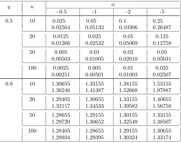
Some numerical values of optimal k for the case of known σ and optimal λ for the case of both parameters of the parent distribution N (0, 1) unknown are presented in Table 1.
Table 1. Optimal values of k (first row) and λ (second row) α q n −0.5 -1 -2 -5 0.5 10 0.025 0.05 0.1 0.25 0.02564 0.05133 0.10306 0.26487 20 0.0125 0.025 0.05 0.125 0.01266 0.02532 0.05069 0.12758 50 0.005 0.01 0.02 0.05 0.00503 0.01005 0.02010 0.05031 100 0.0025 0.005 0.01 0.025 0.00251 0.00501 0.01003 0.02507 0.9 10 1.30655 1.33155 1.38155 1.53155 1.36246 1.41387 1.52668 1.97887 20 1.29405 1.30655 1.33155 1.40655 1.32117 1.34533 1.39582 1.56758 50 1.28655 1.29155 1.30155 1.33155 1.29720 1.30652 1.32549 1.38507 100 1.28405 1.28655 1.29155 1.30655 1.28934 1.29395 1.30324 1.33174
It is obvious that k(n, q, α) → zq as n → ∞. Though numerically
easily confirmed, no analytic proof of the convergence λ(n, q, α) → zq as
n→ ∞ is known to the author.
5. Estimating quantiles of an unknown distribution F from a large nonparametric family F. Let F be the family of all continuous and strictly increasing (on their supports) distribution functions and let
xq(F ) = F−1(q) be the (unique) q-th quantile (quantile of order q) of the
distribution F ∈ F. Let X1:n, X2:n, . . . , Xn:n (X1:n ≤ X2:n ≤ . . . , ≤ Xn:n)
be an ordered sample from an unknown distribution F ∈ F. The sample
size n is assumed to be fixed. The problem is to estimate xq(F ).
As a class T of estimators to be considered we take the class of all es-timators which are equivariant with respect to monotonic transformations
of data and we measure the error of estimation of xq(F ) by an estimator
be found, for example, in Zieli´nski (1999, 2001, 2004). The Linex loss function takes on the form exp{α (F (T ) − q)} − α (F (T ) − q) − 1, α < 0 (Fig. 2). Figure 2. Exp{α(x − q) − α(x − q) − 1} 0.0 0.2 0.4 0.6 0.8 1 0 100 ... ... ... ... ... ... ... ...... ... ... ... ... ... ... ...... ... ... ...... ... ... ...... ...... ... ......... ... ... ... ... ... ... ... ... ... ... ... ... ... ... ... ... ... ... ... ... ... ... ... ...... ...... ...... ...... ...... ...... ...... ...... ...... ...... ...... ...... ...... ...... ...... ...... ...... ... ... ... ... ... ... ... ... ... ... ... ... ... ... ... ... ... ... ... ... ... ... ... ... ... ... ... ... ... ... ... ... ... ... ... ... ... ... ... ... ... ... ... ... ... ... ... ... ... ... ... ... q = 0.9 x α=−10 α=−20 α=−100 • 0.0 0.2 0.4 0.6 0.8 1 0 100 ... ... ... ... ... ... ... ... ... ... ... ... ... ... ... ... ... ... ... ... ... ... ... ... ... ...... ... ... ... ...... ......... ... ... ... ... ... ... ... ... ... ... . ... ... ... ... ... ... ... ... ... ... ... ... ... ... ... ... ... ... ... ... ... ... ... ...... ... ... ...... ...... ...... ...... ...... ...... ...... ...... ...... ...... ...... ...... ...... ...... ......... ... ... ... ... ... ... ... ... ... ... ... ... ... ... ... ... ... ... ... ... ... ... ... ... ... ... ... ... ... ... ... ... ... ... ... ... ... ... ... ... ... ... ... ... ... ... ... ... ... ... ... ... q = 0.5 x α=−10 α=−20 α=−100 •
An estimator T belongs to the class T iff it is of the form T =
XJ(λ):n, where J = J(λ) is a random integer, independent of the
sam-ple X1:n, X2:n, . . . , Xn:n, such that P {J = j} = λj, Pλj = 1, λj ≥ 0
(Uhlmann (1963) for j fixed, Zieli´nski (2004) for J random). Observe that
if the sample comes from a distribution F ∈ F then F (T ) = F (XJ(λ):n) =
UJ(λ):n, where Uj:nis the j-th order statistic from the uniform distribution
U (0, 1). It follows that the risk of the estimator T = XJ(λ):n under the
Linex loss is given by the sum
n
X
j=1
λjR(j, n; q, α)
R(j, n; q, α) = = n! (j−1)!(n−j)! Z 1 0 expα (x−q)−α(x−q)−1xj−1(1−x)n−jdx = e−αq1F1(j, n + 1; α)− j n + 1α + (αq − 1) Here 1F1(j, n + 1; α) = Γ(n + 1) Γ(j)Γ(n − j + 1) Z 1 0 eαttj−1(1 − t)n−jdt
is the confluent hypergeometric function (e.g. Weisstein 1999, Luke 1975). Using the recurrence relation
1F1(j, n + 1; α) −1F1(j − 1, n + 1; α) =
α n + 11
F1(j, n + 2; α)
and taking into account that 1F1(j, n + 1; α) > 0 we conclude that the
first term in R(j, n; q, α) is decreasing in j, the term j/(n + 1) is obviously increasing and in a consequence as a result we obtain that the optimal
estimator is of the form Xj∗:n with j∗ such that
R(j∗, n; q, α) = min
j R(j, n; q, α)
It follows that for j ∈ {1, 2, . . . , n} there exists a unique j∗ such that
R(j∗, n; α, q) < R(j, n; α, q), j 6= j∗
or
R(j∗, n; α, q) = R(j∗+ 1, n; q, α) < R(j, n; q, α), j /∈ {j∗, j∗+ 1}
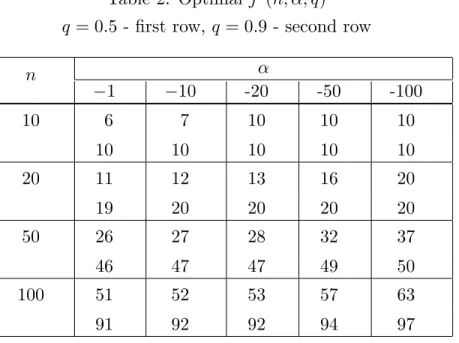
The optimal j∗ can be easily found numerically. Some values of j∗ =
Table 2. Optimal j∗(n, α, q)
q = 0.5 - first row, q = 0.9 - second row α n −1 −10 -20 -50 -100 10 6 7 10 10 10 10 10 10 10 10 20 11 12 13 16 20 19 20 20 20 20 50 26 27 28 32 37 46 47 47 49 50 100 51 52 53 57 63 91 92 92 94 97 References
Abramowitz, M. and Stegun, I.A. (eds). (1972), Handbook of Mathe-matical Functions with Formulas, Graphs, and MatheMathe-matical Tables, New York, Dover
Gradshteyn, I.S., Ryzhik, I.M. (2000): Tables of Integrals, Series, and Products, 6th ed., San Diego, CA, Academic Press
Khindarova, I.N. and Rachev, S.T. (2000): Value at risk: Recent advances.
In: Anastassiou, G. (ed), Handbook of analytic-computational methods in
applied mathematics, Boca Baton, Chapman & Hill/CRC
Yi-Ping Chang, Mingh-Chin Hung, and Yi-Fang Wu (2003), Nonparamet-ric Estimation for Risk in Value-at-Risk Estimator, Communications in Statistics, Simulation and Computation, Vol.32, No.4, pp. 1041-1064 Luke, Y.L. (1975): Mathematical functions and their approsimations, Aca-demic Press
W. Uhlmann (1963), Ranggr¨ossen als Sch¨atzfunktionen, Metrika 7 (1),
Eric W. Weisstein (1999), Confluent Hypergeometric Function of the First
Kind, MathWorld - A Wolfram Web Resource,
http://mathworld.wol-fram.com/ConfluentHypergeometricFunctionoftheFirstKind.html
R. Zieli´nski (1999), Best equivariant nonparametric estimator of a quantile,
Statistics and Probability Letters 45, 79-84.
R. Zieli´nski (2001), PMC-optimal nonparametric quantile estimator,
Statistics 35, 453-462.
R. Zieli´nski (2004), Optimal quantile estimators; Small sample approach,