Creating a switchable optical cavity
with controllable quantum-state
mapping between two modes
Grzegorz Chimczak
1, Karol Bartkiewicz
1,2, Zbigniew Ficek
3,4& Ryszard Tanaś
1We describe how an ensemble of four-level atoms in the diamond-type configuration can be applied to create a fully controllable effective coupling between two cavity modes. The diamond-type configuration allows one to use a bimodal cavity that supports modes of different frequencies or different circular polarisations, because each mode is coupled only to its own transition. This system can be used for mapping a quantum state of one cavity mode onto the other mode on demand. Additionally, it can serve as a fast opening high-Q cavity system that can be easily and coherently controlled with laser fields.
Quantum systems, in which a control of the coherent evolution is possible, are of great importance from a the-oretical and a practical points of view, and therefore, such systems always attract research interest1,2. Systems composed of a cavity and atoms, which are trapped inside this cavity, are such systems because one can easily control the evolution of their quantum state just by illuminating atoms with a laser3–7. Moreover atom-cavity systems provide a versatile environment for engineering complex non-classical states of light8–17. Researchers achieve such high level of control over the evolution of quantum states employing atoms, which can be modelled by few special level schemes. The simplest and frequently considered schemes are three level atoms in Λ and V configurations18–25. The main advantage of these atoms is the possibility of working with the two-photon Raman transition involving an intermediate level, which is populated only virtually during the whole evolution. Since atoms are driven by a classical laser field, the Raman transition takes place only if the laser is turned on. The same idea allows for full control of the system evolution in many other level schemes. Therefore researchers have used and studied intensively many different types of atoms coupled to the cavity mode26–36. There is, however, one important atomic level scheme, which is almost ignored by researchers in the context of atom-cavity systems–a four-level atom in the diamond configuration (a ⬦-type atom, also known as a double-ladder four-level atom). Despite the fact that this level scheme is rich in quantum interference and coherence features37 and has many other applications38–45, to the best of our knowledge there are only few articles about the ⬦-type atom coupled to the quantized field modes46–57.
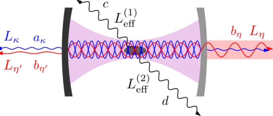
In this paper we study a ⬦-type atom interacting with two quantized cavity modes and two classical laser fields. The quantized field modes are coupled to lower atomic transitions while the classical laser fields are coupled to upper atomic transitions, as depicted in Fig. 1. Here, we show that under certain conditions this system creates effective coupling between two cavity modes of different frequencies or different circular polarisations and its evolution can be described by a simple effective Hamiltonian, and can be easily controlled just by switching the lasers on and off. Moreover, we show that it is possible to increase the effective coupling strength between both modes by using an ensemble of four-level ⬦-type atoms, which interact collectively with both modes. We also present two applications of this system. First of them is a mapping of an arbitrary state of light from one mode onto the other. By mapping we mean an operation, which is defined by the transformation equation
∑ | 〉 ⊗ | 〉 → | 〉 ⊗ ∑ | 〉c k c k
( k k A) 0B 0A ( k k B)58. This operation makes it possible to transfer coherent superpositions of cavity-mode number states from the mode labeled by A to the mode labeled by B. Second application is a device that plays the role of an effective cavity, in which we can change the effective Q factor on demand just by turning the lasers on and off. This device is based on the scheme proposed by Tufarelli et al.59 but it employs ⬦-type atoms 1Faculty of Physics, Adam Mickiewicz University, PL-61-614, Poznań, Poland. 2RCPTM, Joint Laboratory of Optics of Palacký University and Institute of Physics of Academy of Sciences of the Czech Republic, 17. listopadu 12, 772 07, Olomouc, Czech Republic. 3National Centre for Nanotechnology and Advanced Materials, KACST, P.O. Box 6086, Riyadh, 11442, Saudi Arabia. 4Quantum Optics and Engineering Division, Institute of Physics, University of Zielona Góra, Szafrana 4a, Zielona Góra, 65-516, Poland. Correspondence and requests for materials should be addressed to G.C. (email: chimczak@amu.edu.pl)
Received: 20 June 2018 Accepted: 13 September 2018 Published: xx xx xxxx
www.nature.com/scientificreports/
instead of two-level atoms which makes the physics of the described system much richer. Thus, the proposed system has the potential to be more versatile and efficient in quantum information processing than the solutions based on the two-level atoms.
This paper is organized as follows. Firstly, we present the effective Hamiltonian of simple form that gov-erns the evolution of the analyzed complex quantum system and we study conditions under which the effective Hamiltonian can be considered as a good approximation of the general Hamiltonian. Secondly, we investigate the behaviour of the system in two different cases, when lasers are turned off and in the limit of high-intensity laser fields, to show that we can control the effective coupling between two cavity modes just by switching the lasers on and off. Thirdly, we prove using the effective Hamiltonian that the system can perform a state-mapping operation between these two modes. Fourthly, we present the basic idea of the second application of the system, i.e., a fast opening high-Q cavity. Lastly, we discuss in detail the system performance for this second application.
Results
Effective description of the system.
We consider an ensemble of n identical four-level atoms in the dia-mond configuration (Fig. 1) with a ground level |0〉, two non-degenerate intermediate levels |1〉, |2〉, and an upper level |3〉. There are four allowed transitions in this level scheme. The |0〉 ↔ |2〉 transition is coupled to the field mode represented by the annihilation operator a with coupling strength g, while the |0〉 ↔ |1〉 transition is cou-pled to the field mode described by the annihilation operator b with coupling strength g ′. The frequency of the a mode is ω and the frequency of the b mode is ω′. Both field modes are equally detuned from the corresponding transition frequencies by Δ =(E1−E0)/− ′ =ω (E2−E0)/−ω. The upper transitions |1〉 ↔ |3〉 and |2〉 ↔ |3〉 are driven by coherent laser fields of frequencies ν′ and ν, respectively. The coupling strengths between these atomic transitions and the laser fields are denoted by Ω′ and Ω. Both laser fields are detuned from the cor-responding transition frequencies by Δ. Simultaneously, the atom is coupled to all other modes of the EM field, which are assumed to be in the vacuum state. The atom provides an effective coupling between both the modes. Of course, the effective coupling strength depends on the number of atoms n. The higher the number of atoms n, the stronger the coupling becomes. We assume that there are n ≥ 1 identical ⬦-type four-level atoms trapped inside the cavity. The evolution of this composite quantum system is governed by the Hamiltonian, which in the rotating frame is given by∑
σ σ σ σ σ σ σ = Δ + Δ + Δ + Ω + Ω′ + + ′ + . . = † † H ga g b { 2 ( h c )}, (1) k n k k k k k k k 1 11 ( ) 22( ) 33( ) 23( ) 13( ) 02( ) 01( ) where = 1 and σ = | 〉 〈 |ijk i j k( ) denotes the atomic flip operator between states |i〉
k and |j〉k for the k th atom. The
Lindblad operators representing spontaneous transitions from the atomic excited states are given by
γ σ γ σ γ σ γ σ
= ′ = = = ′
L1( )k 01( )k, L2( )k 02( )k, L3( )k 3 23( )k, L4( )k 3 13( )k, (2) where γ, γ′, γ3 and γ′3 are spontaneous emission rates for the respective transitions. For the sake of simplicity, we
assume that Ω, Ω′, g and g ′ are real and non-negative. Similar four-level scheme has been proposed in ref.28. The
Figure 1. Energy levels of an atom in the diamond configuration. Lower atomic transitions are coupled to
quantized field modes with frequencies ω and ω′. Upper transitions are driven by classical laser fields with frequencies ν and ν′.
diamond configuration, however, has the advantage that it allows to use (contrary to level scheme of ref.28) atomic transitions with the highest values of the dipole moment. Of course, the higher the dipole moment, the stronger the effective coupling between the modes is. Using the method of adiabatic elimination (see Methods) we derive the following effective Hamiltonian
δ δ δ
= † + † + † + † + †
Heff 0(a a b b) 1b b 2(a b b a), (3)
where δ0 = −ng2α2, δ1 = n(g2α2 − g′2α1) and δ2 = −ngg′α3, for α1 = ξ(Ω2 − 2Δ2), α2 = ξ(Ω′2 − 2Δ2), α3 = −ξΩΩ′, α4 = −ξΔ2, α5 = ξΔΩ′, α6 = ξΔΩ with ξ = 1/(Δ[Ω2 + Ω′2 − 2Δ2]). This effective Hamiltonian (3) works properly
if populations of all atomic excited states are small (see Alexanian-Bose method in Methods). The effective master equation
∑
ρ= − ρ + ρ − ρ+ρ = i H[ , ]{
L (L )† 1 L †L L †L}
2[( ) ( ) ] , (4) j j j j j j j eff 1 2eff( ) eff( ) eff( ) eff( ) eff( ) eff( ) where γ α α γ α α = ′ + ′ = + ′ L n ga g b L n ga g b [ ], [ ], (5) eff(1) 3 1 eff(2) 2 3
requires more restrictive conditions to work properly, because in its derivation (see Reiter-Sørensen method in Methods) we have neglected the Lindblad operators L k
3( ) and L4( )k, which describe spontaneous emissions from the upper states |3〉k. Therefore, we assume that populations of the atomic intermediate levels (|1〉k and |2〉k) are small
and populations of the upper states |3〉k are small even compared with the intermediate levels, because then
prob-abilities of occurrence of collapses described by L k
3( ) and L4( )k are negligibly small. It is necessary to know condi-tions for the parameters, which make these assumpcondi-tions true. We restrict ourselves only to cases where Ω′g ≈ Ωg′. In these cases the effective master equation works properly if the following conditions are satisfied
λ λ λ λ λ λ
|Δ| gmin nmax
(
〈a a† 〉, 〈b b† 〉)
and max( , , , )2 3 5 6 min( , ),1 4 (6) where gmin = min(g, g ′) and λi are dimensionless expansion parameters (see Alexanian-Bose method in Methodsfor the definition of λi parameters). The expansion parameters λ2, λ3, λ5 and λ6 are associated with operators
acting on the states |3〉k. The smaller they are, the smaller are the populations of the states |3〉k. The expansion
parameters λ1 and λ4 are associated with operators acting only on the states |1〉k and |2〉k. Knowing values of g and
g′ of the chosen physical system we set the value of Δ according to the first condition and then we find
numeri-cally the value of Ω for which the second condition is satisfied. We can always find such value of Ω, because when intensities of classical fields tend to infinity, then expansion parameters λ2, λ3, λ5, λ6 tend to zero. In the following
text we are going to use the effective master eq. (4).
Let us consider the dynamics of the four-level atom in the diamond configuration in the limit of high-intensity classical fields. In the dressed-state approach there is one ground atomic state |0〉 and three excited states
μ φ ψ | 〉 = −Ω| 〉 + Ω′| 〉 | 〉 = Ω′| 〉 + Ω| 〉 + Δ − Ω | 〉 | 〉 = Ω′| 〉 + Ω| 〉 + Δ + Ω | 〉 μ φ ψ ( 1 2 ), (2 1 2 2 ( ) 3 ), (2 1 2 2 ( ) 3 ), (7) R R
where μ, φandψ are normalisation factors and ΩR = (Δ2 + 4Ω2 + 4Ω′2)1/2. Here, there are three allowed
transitions: |0〉 ↔ |μ〉, |0〉 ↔ |φ〉 and |0〉 ↔ |ψ〉, each of which is coupled to both cavity modes (see Alexian-Bose method in Methods). As mentioned above, when intensities of classical fields tend to infinity, then expansion parameters λ2, λ3, λ5, λ6 tend to zero. It means that only two atomic levels, i.e. |0〉 and |μ〉, are enough to describe
the evolution of the system–the four-level atom in the diamond configuration effectively works exactly in the same way as the detuned two-level atom in this regime. Note that the excited bare state |3〉 can be then neglected. It might seem counter-intuitive that high coupling strengths between the atomic upper transitions and the laser fields lead to an effective decoupling of the upper level |3〉 from the system dynamics, but this idea is known and discussed for example in ref.60.
In the limit of high-intensity classical fields one more thing is clearly seen from the first condition in (6)—the effective coupling strength δ2 scales as n. Such behaviour is the well known feature of the collective
dynamics61–63.
When the lasers are turned off then the evolution of the system is still governed by the Hamiltonian (1) but with Ω = Ω′ = 0. The formulas for the effective Hamiltonian given by eq. (3) and the effective operators in this case read as
γ γ
= − Δ † − ′ Δ † = ′ ′ Δ = Δ .
Heff (ng2/ )a a (ng2/ )b b L, eff(1) n g( / ) ,b Leff(2) n g( / )a (8) Here, we can also easily derive more precise expressions, if we perform the adiabatic elimination of excited atomic states assuming from the start that Ω = Ω′ = 0. This approach results in
www.nature.com/scientificreports/
γ γ γ γ γ γ = − Δ Δ + − ′ Δ Δ + ′ = ′ ′ Δ − ′ = Δ − . † † H ng a a ng b b L n g i b L n g i a /4 /4 , /2 , /2 (9) eff 2 2 2 2 2 2 eff(1) eff(2)It is important to note that there is no coupling between the two cavity modes, and therefore, there is no pho-ton transfer when the lasers are turned off. We will refer to this working mode of the system as to the closed mode.
Quantum-state mapping between two cavity modes.
Under certain conditions the evolution of a complex system formed by an ensemble of four-level diamond-type atoms interacting with two quantized field modes can be easily controlled just by switching the lasers on and off. Let us now demonstrate that we can use this system to transfer a given quantum state of one mode (for example a qudit or the Schrödinger′s cat states) to the other mode on demand. It has shown that in special cases, i.e., for coherent states and for qubit states, the Hamiltonian of the form (3) can swap the states of the two modes26,27. Here, we show that it is possible to transfer an arbitrary photonic state.First, we need the formula for the average photon number in the mode represented by the annihilation oper-ator b, assuming that initially this mode is empty, while the mode represented by a is prepared in the Fock state |nph〉. This formula will help us investigate the photon transfer process. We can derive it introducing the
superpo-sition bosonic operator of both field modes
ε ε
= − − .
C 1 a b (10)
We choose such ε that the Hamiltonian (3) can be expressed in the form Heff= −δrC C† , where δ =r δ +δ
(4 22 12 1/2) . Using this form of the Hamiltonian one can derive the formula for the average photon number
δ δ δ
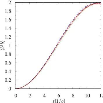
〈b b† 〉 =nph(1− 12/ )sin ( /2)r2 2 rt . (11) In Fig. 2 we plot the average photon number as a function of time. This figure shows that all photons can be transferred from the first mode to the second mode. However, this is possible only if δ1 = 0. We want the state
mapping to be perfect, and therefore, we restrict ourselves to this case only. We can make δ1 ≈ 0 by choosing
val-ues of Ω and Ω′, which are much greater than Δ and satisfy condition Ω′g ≈ Ωg′. If one wants δ1 = 0 then values
of Ω and Ω′ have to be chosen more precisely
Ω′ = (Ω − Δ ′2 2 ) /2g g2 2+ Δ .2 2 (12)
For reference, we also calculate numerically the average photon number using the non-Hermitian Hamiltonian
Figure 2. The average photon number in the b mode as a function of time calculated numerically (solid line)
and given by eq. (11) (dashed line) for one atom n = 1 and (g′, Δ, Ω, Ω′, γ, γ′, γ′′)/g = (1, 11, 55, 55, 1, 1, 1), where g/2π = 10 MHz. At t = 0 the a mode is prepared in the state |2〉A, while the b mode is in a vacuum state.
γ σ γ σ γ σ σ σ σ σ = Δ − ′ + Δ − + Δ − ″ + Ω + Ω′ + + ′ + . . ∼ † † H i i i ga g b ( /2) ( /2) (2 /2) ( h c ), (13) 11 22 33 23 13 02 01
which governs the evolution of this open system during the time intervals when no collapse occurs64,65. We have obtained the Hamiltonian (13) by substituting the relevant symbols in
∑
= −
∼ †
H H i L L
2 j j j (14)
with quantities from eqs (1) and (2) for n = 1. As one can see from Fig. 2, the analytical results are in a remarkable agreement with the numerical solution even for quite considerable values of γ, γ′ and γ′′ (where γ″ =γ3+ ′γ3) as long as parameter regime justifies adiabatic elimination.
From eq. (11) we can infer that the π pulse time is given by the formula
π δ
=
π
t / ,r (15)
from which one can observe one more important feature of the Hamiltonian. It is evident that the time of such π pulse is independent of nph, and thus, we are able to perform the state-mapping operation defined by
|nph〉A ⊗ |0〉B → |0〉A ⊗ |nph〉B. Let us move into the rotating frame, in which the Hamiltonian takes the form
δ δ
= − † + † + † + †
Heff 2(a a b b) 2(a b b a) (16)
and let us assume that the first mode is initially prepared in some interesting quantum state |Ψ 〉 = ∑ | 〉0 k kc kA, while the second mode is empty. Then, by switching the lasers on for tπ, one can map this interesting state onto the
second mode
∑
∑
| 〉 ⊗ | 〉 → | 〉 ⊗ | 〉 . c k 0 0 c k (17) k k A B A k k BIn a frame rotating at different frequency, in which the Hamiltonian takes the form
δ δ
= † + † + † + †
Heff x(a a b b) 2(a b b a), (18)
phase factors appear and the π pulse changes the initial state according to
∑
∑
| 〉 ⊗ | 〉 → | 〉 ⊗ | 〉 φπ c k 0 0 c e k , (19) k k A B A k k i k B ( )where φπ(nph) = −nphπ(δ2 + δx)/(2δ2). Note that for the parameters values used in Fig. 2 δ0 = −2.74 and δ2 = 2.98,
so δ0 ≈ −δ2. For the Hamiltonian (3), δ1 = 0 and large Ω there are no phase factors, because δ0 tends to −δ2 for
large Ω, and thus, the Hamiltonian (3) tends to the form given by eq. (16). The independence of tπ from nph is
crucial for the state-mapping operation. Unfortunately, tπ is independent of nph only in the approximated model
(3), in which we adiabatically eliminated all atomic excited levels. Numerical calculations show that tπ increases
with nph in the more general model of the system given by the Hamiltonian (1) for n = 1. However, as long as
the adiabatic elimination is justified, we can neglect the dependence tπ on nph, as is seen in Fig. 3. It is seen from
Fig. 3 that there are jumps of the value of tπ. These jumps come from the fact that populations of atomic excited
levels oscillate with high frequencies66–68. Thus, there are many local closely-spaced maxima of the population of the desired final state |0〉A ⊗ |nph〉B. Therefore, the global maximum (tπ) changes sometimes discontinuously with
increasing of nph–from one local minimum to the next one. We can neglect these jumps as long as the adiabatic
elimination is justified.
Let us now investigate the effect of γ and γ′ on the state-mapping operation. To this end we need non-Hermitian Hamiltonian, which we obtain by inserting Eq. (3) and the relevant effective rotating frame Lindblad operators (see Reiter-Sørensen method in Methods) into eq. (14). Assuming that Ω Ω′, Δ and δ1 = 0,
this Hamiltonian can be quite well approximated by
δ γ = − − ∼ † † H 2 C C i C C 2 , (20) 2 eff
where the effective dissipation rate is given by
γ = ′ γ′ + ′γ Δ + ′ . ng g g g g g 2 ( ) ( ) (21) eff 2 2 2 2 2 2 2 2
It is clear that the fidelity of the state mapping and the probability that no collapse occurs during this oper-ation are close to one only if the effective dissipoper-ation rate γeff is much less than the effective coupling strength δ2.
For g = g′ and γ = γ′, the expression for the effective dissipation rate takes the simpler form γeff=n g /γ 2Δ2. In this special case, and depend on the ratio γ/Δ. Let us now check this result numerically using the non-Hermitian Hamiltonian
www.nature.com/scientificreports/
∑
γ σ γ σ γ σ σ σ σ σ = Δ − ′ + Δ − + Δ − ″ + Ω + Ω′ + + ′ + . . . ∼ = † † H i i i ga g b {( /2) ( /2) (2 /2) ( h c )} (22) k n k k k k k k k 1 11 ( ) 22( ) 33( ) 23( ) 13( ) 02( ) 01( )First, we have to choose specific values of parameters. The choice of the atom-cavity system determines g, g′,
γ, γ′ and γ′′. For macroscopic cavities g/2π is typically of the order of 10 MHz and γ ranges from about 0.2 g to
g4,36. Let us set g′ = g = 2π⋅10 MHz, γ′ = γ = 2 g and γ′′ = g. The choice of the initial state determines the Fock state |nph〉, to which the state mapping has to be faithful. Let the initial state of the a mode be |Ψ0〉 = (|0〉A + |1〉A + |2〉A
+ |3〉A)/2. If there are four atoms trapped in the cavity, then the detuning has to satisfy Δg 4 3. We set ⋅
Δ = 35 g. Finally, we choose the value of Ω and calculate Ω′ using eq. (12). These values have to be large enough to satisfy the second condition in (6). It is easy to check that for Ω = Ω′ = 175 g this condition is fulfilled, and therefore, adiabatic elimination is justified. For (g′, Δ, Ω, Ω′, γ, γ′, γ′′)/g = (1, 35, 175, 175, 2, 2, 1) and n = 4 we have found that = .0 993 and = .0 885. In the case of one atom trapped in the cavity (n = 1), for the same parameters, we have found that = . 0 995 and = . 0 886. One can see that and are almost the same in the two cases. The only important difference is the time of the state-mapping operation–tπ = 26.5/g and tπ = 105.6/g
for n = 4 and n = 1, respectively. The time of the state mapping in the one-atom case is almost four times larger than that in the four-atom case. This result is in an agreement with eq. (15). We can make tπ smaller in the
one-atom case by setting smaller Δ but then the ratio γ/Δ increases and the dissipation reduces the fidelity and the success probability. For instance, if we set (g′, Δ, Ω, Ω′, γ, γ′, γ′′)/g = (1, 17, 85, 85, 2, 2, 1) in the one-atom case then the time of the state mapping is reduced to tπ = 51.6/g. Then, however the dissipation reduces the fidelity and
the success probability to = .0 979 and = .0 795, respectively.
Quantum-state extraction by fast opening high-Q cavity.
The investigated system can be applied as a fast opening high-Q cavity that can be easily and coherently controlled with classical laser fields. The device is based on similar principles as the setup of Tufarelli et al.59, but it employs four-level atoms in the diamond con-figuration instead of two-level atoms. The main idea of both setups is to couple a high-Q cavity mode to a low-Q cavity mode through atoms. Such a device would be very useful, because on the one hand we need a high Q factor to reach the strong coupling regime4,6,69–74, in which we can generate a complex non-classical state of light trapped inside optical resonator8–17. On the other hand, we need a low Q factor to extract this state from the resonator into a waveguide before it will be distorted by the cavity damping. The device proposed by Tufarelli et al.59 makes it possible to change the effective Q factor. If atoms are absent, there is no coupling between the two modes and the whole system works as an effective high-Q cavity. If we move atoms into the cavity, then photons leak out of the high-Q mode through the low-Q mode and the whole device works as an effective low-Q cavity. Instead of shifting the atoms out of the cavity we can shift atoms out of resonance using a laser and the dynamic Stark effect. As long as the laser illuminates atoms, there is no coupling between modes. Here, we propose to replace two-level atoms by four-level atoms in the diamond configuration. Our modification allows us to use a bimodal cavity,Figure 3. Deviation of tπ(nph) from tπ(1) (in percent) for (g′, Δ, Ω, Ω′)/g = (1, 10, 33, 33) (open squares) and for
(g′, Δ, Ω, Ω′)/g = (1, 30, 100, 100) (solid circles). The second parameter regime justifies adiabatic elimination for
which supports circularly polarised modes of the same or different polarisations and frequencies. Moreover, it requires intense laser light to illuminate atoms only in short time intervals, when we need the coupling between modes. When the laser is switched off, there is no coupling between modes.
Discussion
After the adiabatic elimination of atomic excited states we can restrict our considerations to a simplified model, which does not include atomic variables. Such simplified model makes it easy to take into account all photon losses. To this end, we model the device as two cavity modes, which decay emitting the radiation into five travel-ling modes, as is depicted in Fig. 4. One of these travelling modes is accessible experimentally. This accessible travelling mode can be, for example, a waveguide. Other travelling modes are inaccessible, and thus, provide losses. The photon emissions from both cavity modes (represented by operators a and b) into the inaccessible travelling modes are described by the Lindblad operators: Lη′= η′b, Lκ= κa, Leff(1) and L
eff(2). The photon emis-sion into the accessible travelling mode is described by the Lindblad operator Lη= ηb. Here we assume, unless
explicitly stated otherwise, that the device is working in the open mode, i.e., both lasers are turned on (Ω, Ω′ ≠ 0). We also assume that the quantum state of field was prepared in advance in the mode represented by the operator
a. Under these assumptions, we derived a quantity that describes the quality of the field extracted from the
reso-nator into a waveguide. We refer to this quantity as to the figure of merit of the proposed device (see Methods). Let us now investigate the usefulness of the considered device to extract a field state from the a mode. We assume that there is only one optical cavity. This cavity supports two electromagnetic field modes of different frequencies
ω and ω′ (see Fig. 4). The first of them is considered as the a mode, while the second one as the b mode. Each cavity mirror is described by its radius of curvature r, transmission coefficients T and T′ for the a mode and the b mode, respectively, and loss coefficient L, which is assumed to be the same for both modes. The a mode requires very low values of T and L for both mirrors. To our knowledge, these parameters take the lowest value for the mirror that has been used in the experiment of refs36,75. We set these values in our calculations, i.e., Tsmall = T1 = T2 = T′1 = 1.8 ppm and L = 3.15 ppm, where the subscripts indicate the mirror. The radius of
curva-ture of both mirrors is 50 mm36,75. Now we can vary only the cavity length l and the transmission coefficient T′ 2,
and therefore, we want to plot the figure of merit F as a function of these two quantities. First, we have to choose a concrete realisation of the ⬦-type atom. This kind of atomic level scheme has been investigated experimentally using different atoms. The ⬦-type configuration has been realised using cesium40 and rubidium atoms41–44. From refs76,77 we can infer that it is also possible to obtain the ⬦-type configuration using sodium dimers. We can also choose different levels, which can form the diamond configuration. For example in rubidium atoms we can choose levels (5S1/2, 5P1/2, 5P3/2, 6S1/2)41, (5S1/2, 5P1/2, 5P3/2, 5D3/2)42–44 or (5S1/2, 5P3/2, 6P3/2, 5D5/2)56. Here, we
pro-pose to use a 87Rb atom and its levels |5S
1/2, F = 2, mF = 2〉, |5P3/2,F = 3,mF = 3〉, |6P3/2, F = 3, mF = 3〉 and |6D3/2, F = 3, mF = 3〉 to serve as |0〉, |1〉, |2〉 and |3〉, respectively. This choice determines values of modes frequencies to
be ω/2π = 713.28 THz and ω′/2π = 384.23 THz78. The lifetimes of all used here excited levels can be found in ref.79. It is important that the lifetime of the level |3〉 is longer (τ
3 = 256 ns) than lifetimes of the other excited
levels (τ1 = 112 ns for |1〉 and τ2 = 26.25 ns for |2〉). So our assumption that spontaneous emissions from the
excited level |3〉 can be neglected in calculations is justified not only by small population of this level, but also by
τ3>τ1 and τ3τ2. The spontaneous emissions can take the 87Rb atom from the states |1〉 and |2〉 only to state |0〉.
Hence, it is easy to calculate corresponding spontaneous emission rates: γ/2π = 1.42 MHz and γ′/2π = 6.06 MHz. In principle, the scheme presented here works properly even with only one trapped atom. In real experiments, however, this scheme will require a much larger number of atoms to achieve the figure of merit that is close to unity. In order to compare our scheme with the original scheme of Tufarelli et al.59, we set here the same number of atoms as in ref.59, i.e., n = 1000. Trapping 1000 rubidium atoms and preparing them in the |5S
1/2, F = 2, mF = 2〉
state is possible using fiber-based Fabry-Perot cavities80,81. We have chosen the macroscopic cavity in our consid-erations. A number of atoms trapped inside macroscopic cavities is typically of the order of 10582. Trapping ~1000 atoms also should be possible. Now we can calculate the coupling strength g using
Figure 4. The effective model of the setup and the waveguide. The photon emission from the open cavity into
the waveguide is represented by the operator Lη. All photon losses are modelled by four inaccessible travelling
www.nature.com/scientificreports/
π γ ω = g c V 3 2 , (23) 3 2where c is the speed of light and V is the cavity mode volume given by
π ω
= − .
V cl l r(2 l) /(4 ) (24)
In order to calculate the coupling strength g′ we have to replace ω and γ by ω′ and γ′ in (23) and (24). The cavity damping constants of the considered scheme can be calculated as
κ=c(1−R l R)/( ), η= ′T2 totη / , η′ =(2L+ ′T1 tot) / ,η (25)
where R = 1 − L − Tsmall, = 2L+ ′ + ′T1 T2 and
η = − − − ′ − − ′ . c R L T lR L T 1 (1 ) (1 ) (26) tot 1/4 2 21/4
Finally, we have to fix values of Δ, Ω and Ω′. It is necessary to choose these values carefully. On the one hand, they should be big enough to make adiabatic elimination justified. On the other hand, they cannot be too big, because δ2 and extraction efficiency decrease with increasing Δ. In our computations we set Δ/g = 700 and
Ω/Δ = 5, which justifies adiabatic elimination for cavity states with 〈a a† 〉10. Then Ω′ is given by (12). Now, we can discuss the experimental feasibility of the scheme. In order to do so let us use figure of merit F closely related to the probability of successful operation of the discussed device. Under certain conditions (given explicitly in Methods) F is given as
η η ζ θ ζ θ δ η κ ζ ζ δ η κ ζ ζ = − + − + + + + + F 1 ( ) 2 ( ) 4 ( ), (27) tot 1 1 2 2 2 22 tot 1 2 22 tot 1 2
where ζ1=nγ α′ 32 2g , θ1=nγ α′ 12 2g′ , ζ2=nγα22 2g , θ2=nγα32 2g′ , ηtot = η′ + η. We can plot F as a function of l
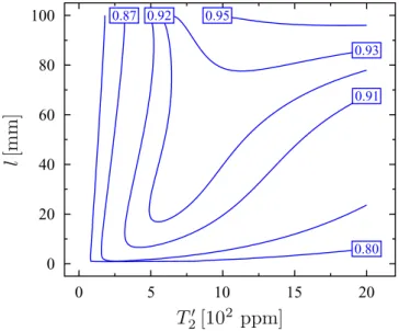
and ′T2. For the parameters given above the formula (27) gives only raw approximation of the figure of merit. Therefore, we have calculated F numerically using its definition (given in Methods), and we have obtained in this way results presented in Fig. 5. As expected, the figure of merit takes the maximum value in the near-concentric regime l ≈ 2r. For l = 99.9 mm and ′T2 = 2000 ppm the figure of merit is equal to 0.97. Unfortunately, the near-concentric configuration of the macroscopic mirrors is extremely sensitive to misalignment, and therefore, it would be difficult or even impossible to achieve such high value of F83. For the confocal configuration l = r, which is the most stable configuration, the figure of merit can be equal to 0.92. This value is still quite high and it is higher than F of the original scheme of Tufarelli et al.59. Of course, we can always increase the figure of merit by increasing n. To show this we plot also the figure of merit for n = 8000. It is seen from Fig. 6 that now F = 0.97 even for the confocal configuration. Form eq. (27) it follows that the figure of merit can be close to one only under the condition δ4 22η κtot( +ζ1+ζ2). Assuming δ1 = 0, this condition can be expressed as:
Figure 5. Figure of merit F as a function of the cavity length l and the transmission coefficient T′2 for 1000
ηtotng2/ ,γ η ng′/ ,γ η′ δ δ κ( / ). (28)
tot 2 tot 2 2
It follows that κ has to be at least two orders of magnitude smaller than δ2. For currently available atom-cavity
systems all these conditions can be satisfied only for a large number of atoms n. Note that F is independent of δ1
in the mentioned regime. Typically, g ≠ g′ in concrete realisations of the four-level atom, and therefore, usually
δ1 ≠ 0. A non-zero value of δ1 decreases F when dissipative rates are too large. It is possible to make δ1 = 0 by
set-ting appropriate value of Ω′, i.e., this one given by eq. (12). From eq. (27), it is seen that such precise setting of Ω′ is not necessary in the regime, in which the figure of merit is close to one. This feature makes choosing values of parameters easier. It is also worth to note that in the regime ΩΔ eq. (12) takes the simpler form Ω′ ≈ Ω ′g g .
Let us now verify the approximate formula (27) for the parameter regime corresponding to the confocal configu-ration with 1000 atoms. By setting l = 50 mm and T′2 = 800 ppm, we get ( , , , , , , ,g g′ Δ Ω Ω′ γ γ γ η′ ″, tot, )/(2 )κ π=
. . . ⋅ −
(0 1, 0 29, 72 8, 364, 989, 1 4, 6 06, 0 6, 0 4, 4 7 10 )3 MHz. These lead to (ζ
1, θ1, ζ2, θ2)/(2π) = (1.3, 2.3, 1.2,
2.5) kHz and δ2/(2π) = 0.14 MHz. As mentioned earlier, the formula (27) is valid if the conditions δ2κ ζ θ ζ θ, , , ,1 1 2 2 and ηtotδ2 are fulfilled. One can see that the first condition is fulfilled. However, the ratio
ηtot/δ2 is only 2.8. Nevertheless, the value of the figure of merit calculated using eq. (27), i.e., F = 0.95 is quite close
to the value F = 0.92 obtained numerically using its definition.
So far, we have investigated the device working in the open mode. Let us now consider this device working in the closed mode. For the device working in the closed mode both lasers are turned off. The effective Hamiltonian derived with Ω = Ω′ = 0 is given by eq. (9). It is seen that there is no interaction between the a mode and the b mode, and therefore, photons do not leak out of the a mode through the b mode. The only destructive role played by atoms trapped inside the cavity is the increase of photon losses caused by the spontaneous emission from the atomic excited state |2〉. The decay of the a mode associated with the atomic spontaneous emission is described by an effective decay rate κγ ≈ nγ(g/Δ)2 [see eq. (8)]. We have found out that for the parameters values used above
(l = 50 mm, T′2 = 800 ppm and n = 1000) this effective decay rate κγ/(2π) = 2.9⋅10−3 MHz is less than the cavity
decay rate associated with the absorption in the mirrors κ/(2π) = 4.7⋅10−3 MHz. Knowing κ
γ, we can take atomic
spontaneous emissions into account just by making the replacement κ→κ′ = κ + κγ.
Conclusion
We have studied a quantum system composed of a ⬦-type atom and an optical cavity supporting two electromag-netic field modes, in which this atom is permanently trapped. We have considered the case, where lower atomic transitions (see Fig. 1) are coupled to the field modes and upper atomic transitions are driven by classical laser fields. We have shown that this complex quantum system can be described by an effective Hamiltonian of the simple form given in eq. (3) if intensities of the lasers fields and the detuning are sufficiently large. In this case the ⬦-type atom intermediates in the interaction between these two modes of the cavity and creates a fully controlla-ble effective coupling between these modes. One can control the effective coupling by lasers, which illuminate the atom. We have also shown that it is possible to obtain enhancement of the effective coupling of a factor n by trapping an ensemble of n ⬦-type atoms inside the cavity. We have presented two examples of applications of this system. The first application is a state transfer from one quantized mode to another. We have shown that the time of the state transfer is independent of the number of photons. Thus, it is possible to map a quantum state of one mode onto the other mode. As the second application of the system, we have presented a device which can be switched on demand to perform either as a low-Q cavity, or as a high-Q cavity. The ⬦-type atoms allow for fast switching between these two working modes just by switching the lasers on and off. Moreover, ⬦-type atoms
Figure 6. Figure of merit F as a function of the cavity length l and the transmission coefficient T′2 for 8000
www.nature.com/scientificreports/
make this device to be especially well suited for a bimodal cavity, which supports circularly polarised modes of the same or different polarisations and frequencies.
Methods
Reiter-Sørensen method.
Initially, all atoms are prepared in the ground state. An atom can be found in one of the excited states, only if it absorbs a single photon. We want to achieve an effective coupling between field modes and no coupling between the modes and atoms. Therefore, the atomic excited states have to be populated only virtually. In this case, we can adiabatically eliminate the atomic excited states and use in calculations an effective Hamiltonian for the ground state subspace. To this end, we use the effective operator formalism for open quantum systems described in ref.84. Let us consider the single atom case first. The Hamiltonian describing a single atom can be easily obtained by simplifying eq. (1) and it readsσ σ σ σ σ σ σ
= Δ + Δ + Δ + Ω + Ω′ + † + ′ † + . . .
H 11 22 2 33 ( 23 13 ga 02 g b 01 h c ) (29)
The Lindblad operators representing spontaneous transitions from the atomic excited states are given by
γ σ γ σ γ σ γ σ
= ′ = = = ′
L1 01, L2 02, L3 3 23, L4 3 13, (30)
where γ, γ′, γ3 and γ′3 are spontaneous emission rates for the respective transitions. The master equation of
Kossakowski-Lindblad form describing the evolution of this system is then given by
∑
ρ= − ρ + ρ ρ ρ − + . = i H[ , ] L L† 1 L L† L L† 2( ) (31) j 1 j j j j j j 4The effective-operator formalism for open quantum systems84 reduces eq. (31) to an effective master equa-tion, where the dynamics is restricted to the atomic ground state only. In order to apply the effective-operator formalism, we need to provide: the Lindblad operators, the Hamiltonian in the exited-state manifold He, the
ground-state Hamiltonian Hg (here Hg = 0.), and the perturbative (de-)excitations of the system V+ (V−). These
are given by σ σ σ σ σ σ σ σ σ = Δ + Δ + Δ + Ω + Ω′ + . . = + ′ = + ′ . − + † † H V ga g b V ga g b 2 ( h c ), , (32) e 11 22 33 23 13 02 01 20 10
The effective Hamiltonian and collapse operators can be derived using formulas84
=− − − + − † ++ H 1V H H V H 2 [ ( ) ] , (33) eff NH1 NH1 g = − + Lj L H V , (34) j eff( ) NH1 where
∑
= − † . H H i L L 2 j j j (35) NH eAssuming that all spontaneous emission rates are negligibly small compared with Ω, Ω′ and Δ we can approx-imate H− NH1 by α σ α σ α σ σ α σ α σ σ α σ σ ≈ + + + + + + + + − HNH1 1 11 2 22 3 12( 21) 4 33 5 13( 31) 6 23( 32), (36) where α1 = ξ(Ω2 − 2Δ2), α2 = ξ(Ω′2 − 2Δ2), α3 = −ξΩΩ′, α4 = −ξΔ2, α5 = ξΔΩ′, α6 = ξΔΩ with ξ = 1/
(Δ[Ω2 + Ω′2 − 2Δ2]). From the combined eqs (33) and (36) we derive the effective Hamiltonian
δ δ δ
= † + † + † + † + †
Heff 0(a a b b) 1b b 2(a b b a), (37)
where δ0 = −g2α2, δ1 = g2α2 − g′2α1 and δ2 = −gg′α3. By inserting eq. (36) into eq. (34) we obtain the effective
Lindblad operators
γ α α γ α α
= ′ + ′ = + ′ .
Leff(1) [ 3ga 1g b L], eff(2) [ 2ga 3g b] (38) Unfortunately, deriving the expressions for operators Leff(3) and Leff(4) is more challenging than deriving Leff(1) and
Leff(2). First of all, the action of the operators L3 and L4 takes the system state to one of the excited states |1〉 or |2〉,
while all the excited states should be populated only virtually. In the single atom case after spontaneous emission from the excited state |3〉 it is necessary to reset the device, otherwise it will not work properly. Second, the effec-tive operator formalism assumes that the excited states decay to the ground states only. We circumvent these obstacles by choosing such values of parameters that probabilities of occurrence of collapses described by L3 and L4 are negligibly small. We will give later conditions for the parameters, which allow us to neglect L3 and L4. Using
∑
ρ= − ρ + ρ − ρ+ρ . = i H[ , ]{
L (L )† 1 L †L L †L}
2[ ) ( ) ] (39) j j j j j j j eff 1 2eff( ) eff( ) eff( ) eff( ) eff( ) eff( )
Alexanian-Bose method.
Using the effective operator formalism and assuming that the upper level |3〉 can be neglected, we have obtained all needed formulas. Unfortunately we still do not know the limits in which these approximations are valid. In order to determine the limits we derive the effective Hamiltonian (3) using another method — a perturbative unitary transformation85. An incidental bonus is that this method provides new insights into the dynamics of the four-level atom in the diamond configuration. Let us start by decomposing the Hamiltonian (29) into two parts= + H H0 H ,1 (40) where σ σ σ σ σ = Δ + Δ + Δ + Ω + Ω′ + . . . H0 11 22 2 33 ( 23 13 h c ) (41)
Diagonalizing H0 in the basis {|1〉, |2〉, |3〉} leads to the dressed states energies
Δ, (3Δ − ΩR)/2, (3Δ + ΩR)/2, (42)
and the semiclassical dressed states μ φ ψ | 〉 = −Ω| 〉 + Ω′| 〉 | 〉 = Ω′| 〉 + Ω| 〉 + Δ − Ω | 〉 | 〉 = Ω′| 〉 + Ω| 〉 + Δ + Ω | 〉 μ φ ψ ( 1 2 ), (2 1 2 2 ( ) 3 ), (2 1 2 2 ( ) 3 ), (43) R R where ΩR = (Δ2 + 4Ω2 + 4Ω′2)1/2, μ = (Ω2 + Ω′2)−1/2, φ = (2ΩR(ΩR − Δ))−1/2 and ψ = (2ΩR(ΩR + Δ))−1/2.
Now, using the new basis {|0〉, |μ〉, |φ〉, |ψ〉}, we express the Hamiltonian (29) as
σ σ σ σ σ σ σ σ σ = Δ + Δ − Ω + Δ + Ω + Ω′ − Ω + Ω − ′Ω − ′Ω′ + ′Ω′ + . . . μμ φφ ψψ μ μ φ φ ψ ψ μ μ φ φ ψ ψ † † † † † † H g a g a g a g b g b g b (3 )/2 (3 )/2 ( 2 2 2 2 h c ) (44) R R 0 0 0 0 0 0
Now we can eliminate atomic excited states |μ〉, |φ〉 and |ψ〉. To this end, we introduce a unitary transformation85 = U exp( ),S (45) where λ σ σ λ σ σ λ σ σ λ σ σ λ σ σ λ σ σ = − + − + − + − + − + − μ μ φ φ ψ ψ μ μ ϕ φ ψ ψ † † † † † † S a a a a a a b b b b b b ( ) ( ) ( ) ( ) ( ) ( ) (46) 1 0 0 2 0 0 3 0 0 4 0 0 5 0 0 6 0 0
and λi are dimensionless parameters such that λ 〈 〉i a a† and λ 〈 〉i b b† are very small compared to 1. These
parameters will play the role of expansion parameters associated with respective excited states. For example, λ1
and λ4 are associated with the state |μ〉 (see eq. (46)).
We transform each operator in (44) using the Baker–Hausdorf lemma
′ = − = + + + …
X e XeS S X [ , ]S X (1/2!)[ , [ , ]]S S X (47)
If we choose λ1 = μgΩ′/Δ, λ2 = 4 gΩ/(3Δ − Ωφ R), λ3 = 4 gΩ/(3Δ + Ωψ R), λ4 = μg′Ω/Δ, λ5 = 4 g′Ω′/φ
(3Δ − ΩR), λ6 = 4 g′Ω′/(3Δ + Ωψ R) then terms which are linear in the field operators vanish in the transformed
Hamiltonian. If we moreover drop all terms much smaller than λ Δ12 then we obtain the effective Hamiltonian (3). Note that both methods, i.e. Reiter-Sørensen method and Alexanian-Bose method, give exactly the same formula for the effective Hamiltonian, despite the fact that both are just approximations.
It is also worth to note that the parameters λi are given by the ratios of the effective coupling constants to the
dressed state energies. The dressed state energies play the role of detunings in this dressed-state approach. So,
λi1 means that the corresponding excited state is very far off resonance from the ground atomic state |0〉, and thus, its population is small. For instance, the smaller λ1 and λ4 are, the smaller is the population of the state |μ〉.
Knowing this we can obtain the conditions (6).
The multi-atom case.
Let us now generalise the effective Hamiltonian to the case of n identical atoms trapped inside the cavity. For the sake of simplicity, we assume here that coupling strengths g and g ′ are the same for each atom in the ensemble. Note, however, that every atom in a Bose-Einstein condensate indeedwww.nature.com/scientificreports/
experiences an identical coupling to the cavity mode59. The evolution of this multi-atom system is represented by the Hamiltonian
∑
σ σ σ σ σ σ σ = Δ + Δ + Δ + Ω + Ω′ + + ′ + . . . = † † H { 2 ( ga g b h c )} (48) k n k k k k k k k 1 11 ( ) 22( ) 33( ) 23( ) 13( ) 02( ) 01( )Let us derive the effective Hamiltonian by using Alexanian-Bose method. To this end we rewrite the Hamiltonian (48) as
∑
σ σ σ σ σ σ σ σ σ = Δ + Δ − Ω + Δ + Ω + Ω′ − Ω + Ω − ′Ω − ′Ω′ + ′Ω′ + . . μμ φφ ψψ μ μ φ φ ψ ψ μ μ φ φ ψ ψ = † † † † † †}
{
(
)
H g a g a g a g b g b g b (3 )/2 (3 )/2 2 2 2 2 h c (49) k n k k k k k k k k k 1 ( ) R ( ) R ( ) 0( ) 0( ) 0( ) 0( ) 0( ) 0( ) and introduce a unitary transformation U = exp(S), where
∑
λ σ σ λ σ σ λ σ σ λ σ σ λ σ σ λ σ σ = − + − + − + − + − + − . μ μ φ φ ψ ψ μ μ φ φ ψ ψ = † † † † † †{
}
S a a a a a a b b b b b b ( ) ( ) ( ) ( ) ( ) ( ) (50) k n k k k k k k k k k k k k 1 1 0 ( ) 0( ) 2 ( )0 0( ) 3 ( )0 0( ) 4 0( ) ( )0 5 ( )0 0( ) 6 ( )0 0( ) If we set λ1 = μgΩ′/Δ, λ2 = 4 gΩ/(3Δ − Ωφ R), λ3 = 4 gΩ/(3Δ + Ωψ R), λ4 = μg′Ω/Δ, λ5 = 4 g′Ω′/φ(3Δ − ΩR), λ6 = 4 g′Ω′/(3Δ + Ωψ R), assume that the conditions (6) are satisfied and drop all terms much smaller
than λ Δ12 then the transformed Hamiltonian takes the form
∑
σ β∑
σ∑
σ β∑
σ∑
σ∑
σ ′ = + + + + . . μ μ μ φ ψ = = = = = = H H h c , (51) k n k k n k k n k k n k k n k k n k eff 100 ( ) 1 1 0 ( ) 10 ( ) 2 1 0 ( ) 10 ( ) 10 ( )where Heff is the effective Hamiltonian (37) describing the evolution of the system in the single-atom case, β1 = g2g′2/(Δ(g2 + g′2)) and β = ′2 gg g( 2− ′g2)/( 2 (Δg2+ ′g2)). Initially all atoms are prepared in the ground state. It is seen that there is no operator in the Hamiltonian (51), which can change this atomic state. Hence all atoms remain in their ground state during the evolution. Therefore we can drop all terms describing excitation exchange between different atoms, i.e., terms containing operators σ σmi
lj
0 ( )
0( ), where m, l = μ, ψ, φ. Of course, we can also drop all terms containing operators σμμ( )k. Then we obtain
Π σ
′ = =
H nHeff kn1 00( )k, (52)
So, in this more general case the effective Hamiltonian is still given by eq. (37), but with
δ0= −ng2α2, δ2= −ngg′α3, andδ1=n g( 2α2− ′g2α1). (53) Let us also derive the effective Hamiltonian using the Holstein-Primakoff transformation86—a standard method in the study of multi-atom systems. We start from the Hamiltonian (49). As mentioned earlier, only two atomic levels, i.e. |0〉 and |μ〉, are enough to describe the evolution of the system in the limit of high-intensity classical fields (see Results). Therefore we assume that the conditions (6) are satisfied and we approximate the Hamiltonian (49) by
∑
σ∑
σ∑
σ = Δ + Ω′ − ′Ω + . . μ μ μ μ = = = † † H g a g b 2k h c , (54) n k k n k k n k 13 ( ) 10 ( ) 10 ( ) where σk =σμμk −σk3( ) ( ) 00( ). Next, we introduce the operators Sz=2−1∑kn=1 3σ( )k, S−= ∑kn=1 0σ( )μk, S+= ∑kn=1 0σμ( )k and
rewrite the Hamiltonian as
= Δ + μ Ω′ † −− μ ′Ω †−+ . . .
H Sz (g a S g b S h c ) (55)
Now we can use the Holstein-Primakoff approximation defined by
= − † −= − † ≈ += † − † ≈ †.
S n c c S n c c n c nc S nc c c n nc
2 , (1 / ) , and (1 / ) (56)
z 1/2 1/2
The Hamiltonian can be written in terms of a bosonic operator c as
= −Δ † + μ Ω′ † − μ ′Ω † + . . .
By assuming that the conditions (6) are satisfied we also assume that the average number of bosonic excita-tions 〈 〉c c is small. Thus we can adiabatically eliminate the bosonic operator c. To this end, we derive formula for †
c from =c i H c[ , ]=087. In this way we obtain
= μ Ω′ − μ ′Ω Δ.
c ( g na g nb)/ (58)
Substituting eq. (58) into the Hamiltonian (57) results in
δ δ δ
= + + + +
∼ † † † † †
Heff 0(a a b b) 1b b 2(a b b a), (59)
where δ0=ng2Ω′2ξ, δ1=n g( ′ Ω −2 2 g2Ω′2)ξ, δ2= −ngg′ΩΩ′ξ and ξ = 1/( (Δ Ω + Ω′2 2)).
The effective Hamiltonian (59) is in agreement with the effective Hamiltonian (3) in the limit of high-intensity classical fields. In order to show this agreement we have calculated numerically the average photon number in the mode represented by the annihilation operator b for an ensemble of 9 atoms using both these effective Hamiltonians and the general Hamiltonian (48). We have assumed that initially the b mode is in a vacuum state, while the a mode is prepared in the state |2〉A and all atoms are prepared in their ground state. The values of the
parameters are chosen such that the conditions (6) are satisfied. It is seen from Fig. 7 that the general Hamiltonian (48) describing the multi-atom case is well approximated by both effective Hamiltonians.
Interaction with an external field.
The two cavity modes interact according to the effective Hamiltonian (3), which in a frame rotating at δ0 takes the form Heff=δ1b b† +δ2(a b† +b a† ). The photon emission from the mode, represented by b, into the waveguide is described by the Lindblad operator Lη= ηb. The absorption inthe mirrors for this mode is modelled as the photon emission into an inaccessible mode and described by
η
= ′
η′
L b. The losses in the mirrors for the a mode are taken into account in the same manner. The photon
absorption from the a mode is described by the operator Lκ= κa. Although the simplified model does not
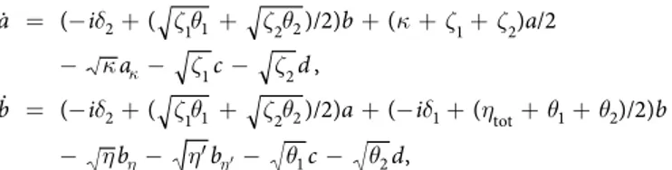
include atomic variables, spontaneous emissions from the excited atomic states |1〉 and |2〉 are taken into account by assuming that there are two inaccessible travelling modes, into which photons from both modes can be emit-ted in the way described by the Lindblad operators Leff(1) and Leff(2). The device working in the open mode has to transfer the state of the a mode to the waveguide. In order to calculate a quantity, which measures how close the output field into waveguide is to the initial a mode field, it is necessary to describe the interaction of the quantum system with the accessible travelling mode. To this end, we use the input-output theory88–90, because it is perfectly suitable for the scheme illustrated in Fig. 4. We have followed the treatment of ref.89 to derive the Heisenberg-Langevin equations for this scheme. These equations take the form
Figure 7. The average photon number in the b mode calculated numerically using the general Hamiltonian (48) (solid curve), the effective Hamiltonian (3) (dashed curve) and the effective Hamiltonian (59) (dotted curve). The parameters regime is (g′, Δ, Ω, Ω′)/g = (1, 34, 180, 180), where g/2π = 10 MHz and the number of atoms is set to 9.
www.nature.com/scientificreports/
δ ζ θ ζ θ κ ζ ζ κ ζ ζ δ ζ θ ζ θ δ η θ θ η η θ θ = − + + + + + − − − = − + + + − + + + − − ′ − − κ η η′ a i b a a c d b i a i b b b c d ( ( )/2) ( ) /2 , ( ( )/2) ( ( )/2) , (60) 2 1 1 2 2 1 2 1 2 2 1 1 2 2 1 tot 1 2 1 2where aκ(t), bη′(t), c(t) and d(t) are output field operators of inaccessible travelling modes, bη(t) is the output field
operator of the waveguide mode and ζ1=nγ α′ 32 2g , θ =nγ α′ g′
1 12 2, ζ2=nγα22 2g , θ2=nγα32 2g′, ηtot = η′ + η. The
matrix form of eq. (60) is given by
= − v Mv v ,out (61) with κ ζ ζ ζ θ ζ θ δ ζ θ ζ θ δ η θ θ δ ≡ + + + − + − + + − M i i i 2 2 2 2 , (62) 1 2 1 1 2 2 2 1 1 2 2 2 tot 1 2 1
where v = [a, b]T and = κ + ζ + ζ η + η′ + θ + θ
κ η η′
vout [ a 1c 2d, b b 1c 2d]T.
Figure of merit.
Now, we can follow closely the treatment of Tufarelli et al.59 to get the figure of merit of the scheme. First, we have to define the bosonic operator for the waveguide field travelling away from the device∫
τ τ τ≡ ∞ η
fout u b( ) ( ) ,d (63)
0 with u(τ) being a temporal profile of the form
∫
τ τ ≡ | | . τ τ − ∞ − u e e d ( ) [ ] [ ] (64) M M 1,2 0 1,22Next, we introduce the bosonic operator hext representing all inaccessible travelling modes. We do not need to
know the specific form of hext in our calculations. Then we can relate the annihilation operator a at the time t = 0
to the output modes using the formula
= − − a(0) Ffout 1 Fhext, (65) where
∫
η τ = ∞| − τ | . F [e M] d (66) 0 1,2 2It is worth to note the similarity between eq. (65) and a unitary transformation representing a beam splitter of transmittance F. This similarity allows us to consider an abstract beam splitter described by relations
= − −
a(0) Ffout 1 Fhext, (67)
= − + .
avac(0) 1 Ffout Fhext (68)
The abstract mode avac(0) must be empty, because the total excitation number has to be conserved, i.e., the
initial number of photons inside the a mode has to be equal to the total number of photons inside outgoing modes
fout and hext. Using the abstract beam-splitter model of the device it is easy to get formula for fout:
= + − .
fout Fa(0) 1 Favac(0) (69)
The parameter F satisfies ≤ ≤0 F 1 and, as it is easy to see from eq. (69), it can work as a figure of merit, because as F gets closer to one, the output field fout gets closer to the initial field a(0). This fact is especially clearly
seen in the Schrödinger picture59
ρ =e −F ρ, (70)
out (1 )0
where ρ0 is the initial state of the a mode, ρout is the final state of the fout mode and the Liouvillian is given by
ρ= 1 a aρ †−a a† ρ−ρa a† .
In order to investigate how well the initial quantum state can be extracted from the cavity using the device presented in Fig. 4, we have to express the figure of merit F as a function of parameters of this device. It can be done using the method presented in ref.59. First, we express the figure of merit as
η = F X1,2,2,1( ),M (72) where ( )M =
∫
∞[e−Mτ] [e−M†τ] dτ (73) 1,2,2,1 0 1,2 2,1is an element of the tensor . We can express this tensor in the matrix form as
∫
τ= ∞ − τ⊗ − †τ
X M( ) e M e M d , (74)
0
where ⊗ indicates the Kronecker product. Since ( ) is the solution to a Sylvester equation, we can obtain all M
elements of ( )M just by solving linear system of equations
⊗ + ⊗ † = ⊗
M I M M I M I I
( ) ( ) ( )( ) , (75)
where I indicates the 2 × 2 identity matrix. In this way we derive the formula for 1,2,2,1( )M, which we insert into
eq. (72). Unfortunately, the obtained expression is too complex to be useful, and thus, it is necessary to resort to further approximations. If we assume that ηtotδ2κ ζ θ ζ θ, , , ,1 1 2 2 then the figure of merit can be well approximated by η η ζ θ ζ θ δ η κ ζ ζ δ η κ ζ ζ = − + − + + + + + . F 1 ( ) 2 ( ) 4 ( ) (76) tot 1 1 2 2 2 22 tot 1 2 22 tot 1 2
References
1. Bo, F. et al. Controllable oscillatory lateral coupling in a waveguide-microdisk-resonator system. Sci. Rep. 7, 8045 (2017). 2. Liu, Y.-L. et al. Controllable optical response by modifying the gain and loss of a mechanical resonator and cavity mode in an
optomechanical system. Phys. Rev. A 95, 013843 (2017).
3. McKeever, J. et al. Deterministic generation of single photons from one atom trapped in a cavity. Science 303, 1992–1994 (2004). 4. Boozer, A. D., Boca, A., Miller, R., Northup, T. E. & Kimble, H. J. Reversible state transfer between light and a single trapped atom.
Phys. Rev. Lett. 98, 193601 (2007).
5. Weber, B. et al. Photon-photon entanglement with a single trapped atom. Phys. Rev. Lett. 102, 030501 (2009).
6. Nölleke, C. et al. Efficient teleportation between remote single-atom quantum memories. Phys. Rev. Lett. 110, 140403 (2013). 7. Hacker, B., Welte, S., Rempe, G. & Ritter, S. A photon–photon quantum gate based on a single atom in an optical resonator. Nature
536, 193 (2016).
8. Larson, J. Scheme for generating entangled states of two field modes in a cavity. J. Mod. Opt. 53, 1867–1877 (2006). 9. Prado, F. O. et al. Atom-mediated effective interactions between modes of a bimodal cavity. Phys. Rev. A 84, 053839 (2011). 10. Domokos, P., Brune, M., Raimond, J., Raimond, J. & Haroche, S. Photon-number-state generation with a single two-level atom in a
cavity: a proposal. EPJ D 1, 1–4 (1998).
11. Savage, C. M., Braunstein, S. L. & Walls, D. F. Macroscopic quantum superpositions by means of single-atom dispersion. Opt. Lett.
15, 628–630 (1990).
12. Rong-Can, Y., Gang, L., Jie, L. & Tian-Cai, Z. Atomic n 00 n state generation in distant cavities by virtual excitations. Chin. Phys. B
20, 060302 (2011).
13. Nikoghosyan, G., Hartmann, M. J. & Plenio, M. B. Generation of mesoscopic entangled states in a cavity coupled to an atomic ensemble. Phys. Rev. Lett. 108, 123603 (2012).
14. Liu, K., Chen, L.-B., Shi, P., Zhang, W.-Z. & Gu, Y.-J. Generation of noon states via raman transitions in a bimodal cavity. Quantum
Inf Process 12, 3057–3066 (2013).
15. Bougouffa, S. & Ficek, Z. Atoms versus photons as carriers of quantum states. Phys. Rev. A 88, 022317 (2013).
16. Xiao, X.-Q., Zhu, J., He, G. & Zeng, G. A scheme for generating a multi-photon noon state based on cavity qed. Quantum Inf Process
12, 449–457 (2013).
17. Liu, Q.-G. et al. Generation of atomic noon states via adiabatic passage. Quantum Inf Process 13, 2801–2814 (2014).
18. Imamoglu, A. et al. Quantum information processing using quantum dot spins and cavity qed. Phys. Rev. Lett. 83, 4204–4207 (1999). 19. Miranowicz, A. et al. Generation of maximum spin entanglement induced by a cavity field in quantum-dot systems. Phys. Rev. A 65,
062321 (2002).
20. Boozer, A. D., Boca, A., Miller, R., Northup, T. E. & Kimble, H. J. Reversible state transfer between light and a single trapped atom.
Phys. Rev. Lett. 98, 193601 (2007).
21. Härkönen, K., Plastina, F. & Maniscalco, S. Dicke model and environment-induced entanglement in ion-cavity qed. Phys. Rev. A 80, 033841 (2009).
22. Cheng, J., Han, Y. & Zhou, L. Pure-state entanglement and spontaneous emission quenching in a v-type atom–cavity system. J. Phys.
B 45, 015505 (2012).
23. Zhang, L.-H., Yang, M. & Cao, Z.-L. Directly measuring the concurrence of atomic two-qubit states through the detection of cavity decay. EPJ D 68, 109 (2014).
24. Casabone, B. et al. Enhanced quantum interface with collective ion-cavity coupling. Phys. Rev. Lett. 114, 023602 (2015).
25. Dong, P., Liu, J., Zhang, L.-H. & Cao, Z.-L. Direct measurement of the concurrence of spin-entangled states in a cavity–quantum dot system. Physica B 495, 50–53 (2016).
26. Lin, G.-W., Zou, X.-B., Ye, M.-Y., Lin, X.-M. & Guo, G.-C. Quantum swap gate in an optical cavity with an atomic cloud. Phys. Rev.
A 77, 064301 (2008).
27. Shao, X.-Q., Chen, L. & Zhang, S. One-step implementation of a swap gate with coherent-state qubits via atomic ensemble large detuning interaction with two-mode cavity quantum electrodynamics. J. Phys. B 41, 245502 (2008).
28. Sharypov, A. V. & He, B. Generation of arbitrary symmetric entangled states with conditional linear optical coupling. Phys. Rev. A