The Henryk Niewodniczański Institute of Nuclear Physics Polish Academy of Sciences Department of Complex Systems Theory
Multiscale characteristics of linear and
nonlinear cross-correlations in financial
markets
Marcin Forczek
This thesis was done under the supervision of dr hab. inż. Paweł Oświęcimka
Acknowledgements
I am profoundly indebted to my supervisor, dr hab. inż. Paweł Oświęcimka, who was very generous with his time and knowledge and assisted me in each step to complete the thesis. I would also like to thank dr hab. Jarosław Kwapień for his remarks and guidance in writing the thesis. Last but not least, I would like to thank prof. dr hab. Stanisław Drożdż, Head of the Department of Complex Systems Theory, for his continued and friendly support throughout my studies.
1
1 INTRODUCTION ... 2
2 STATISTICAL PROPERTIES OF FINANCIAL DATA ... 7
2.1 Models of financial markets ... 7
2.2 Probability distributions of returns ... 11
2.2.1 The foreign exchange market (FX) ... 12
2.2.2 DJIA ... 20
2.3 Autocorrelations and time cross-correlations ... 23
2.3.1 DJIA ... 24
2.3.2 FX market ... 27
3 FRACTAL AND MULTIFRACTAL FORMALISM ... 33
3.1 General properties of fractal sets ... 35
3.2 Fractal dimensions ... 38
3.3 Multifractals and the singularity spectrum ... 41
4 MULTIFRACTAL ANALYSIS OF TIME SERIES ... 44
4.1 The MF-DFA (Multifractal Detrended Fluctuation Analysis) multifractal method ... 45
4.1.1 Analysis of foreign exchange market data ... 50
4.1.1.1 Base currencies ... 50
4.1.1.2 Deviations from the triangular relation ... 55
4.1.1.3 Cross exchange rates– the effect of the number of currencies on the f(α) spectrum width ……….57
4.1.2 Analysis of stock market data ... 60
4.2 The Wavelet Leaders method ... 62
4.3 Multifractal Cross-Correlation Analysis (MFCCA ) ... 67
4.3.1 The foreign exchange market ... 74
4.3.2 The stock market ... 79
4.4 Determination of the cross-correlation coefficient 𝝆𝒒 for time series ... 81
5 NETWORK ANALYSIS OF THE FINANCIAL DATA – MST TREES ... 88
5.1 The 100 largest American companies ... 94
5.2 The 100 smallest American companies ... 103
6 SUMMARY AND CONCLUSIONS ... 111
7 BIBLIOGRAPHY ... 118
2
1 Introduction
With his work "An Inquiry into the Nature and Causes of the Wealth of Nations" published in 1776 [1], the Scottish philosopher and thinker Adam Smith laid foundations for economics as a separate branch of science. In the above-mentioned work, he used the term "invisible hand" meaning a mechanism that directs individual consumers so that their actions are the most beneficial to the whole of society. Although being commonly known and widely covered in the literature, this problem has not been to date put into mathematical formulas in a manner that would enable the market as a whole to be described precisely. This effect is a classic example of an emergent phenomenon, i.e. such a characteristic or property of a system, which has occurred in the system under examination, and which was never previously observed at the level of the individual system components. Phenomena of this type are characteristic of complex systems, where, due to a large number of nonlinear interactions between the elements of the system, evolving structures appear, which cannot be derived from the components in a simple manner. Looking from this perspective on financial markets in a broad sense, one can notice that they perfectly fit into the concept of complex systems. Starting from individual investors in the financial markets or individuals in their households, whose behavior can be described at best in a collective manner, it cannot be determined exactly in which direction the share prices or the domestic economy will, respectively, evolve in the future.
Due to the fact that financial markets have in recent years been supplying a vast amount of information that is readily available at a relatively low cost, more and more researchers from branches of science other than economics are being concerned with market analysis. Since 1973, when currency trading started, the financial institutions have been active round the clock [2]. Until 1995, there had been a nearly 80-fold increase in the volume of transactions, and even more dynamic growth of trade had taken place in the market of derivative financial instruments. A breakthrough in the development of financial market research occurred in 1980 when the capability to make transactions electronically was introduced, which, in turn, allowed the collection of huge amounts of data that became the subject of various analyses. To get an idea of how big and complex system are the financial markets in terms of the number of components, it is sufficient to mention that only in 2013 the two world's largest stock exchanges (NYSE, NASDAQ) traded nearly $12 trillion worth of shares, while the
3
daily number of NYSE stock exchange transactions amounts to almost 2.5 million orders1. Bloomberg, the world's largest supplier of information systems in the area of finances, has nearly 320.000 information terminals in 73 countries, which are used each day by millions of users. Roughly from the mid-1990s, the research activity of physicists in the field of economics began to be increasingly clearly visible. This activity made a bridge between financial mathematics, regarded by many as a kind of technical analysis, and the traditional approach used by financiers. The observation and recording of movements in the financial markets has enabled the construction of theoretical models needed for their description and practical verification.
The first attempts to describe the financial markets, known in the literature, date from the beginning of the last century, when Louis Bachelier, a French mathematician, proposed the random walk as the first model of the dynamics of the share price [3] , based on the assumption that price fluctuations are subject to Gauss distribution. His doctoral thesis entitled "The Theory of Speculation" [3] laid foundations for the development of financial mathematics, and the model described therein has still been used in economics, even though it does not completely correctly describe the dynamics of share prices. It is now known that the probability density distributions of financial fluctuations in the range of large financial events disappear very slowly (fat tails) [4; 5], which in practice means that the probability of rare events is greater than it would appear from the normal distribution. One of the first, who drew attention to this fact, was Benoit Mandelbrot. He formulated the thesis that the distributions of returns should be described with the stable Levy distribution [6]. As has turned out, however, this model does not fully reflect reality, because the tails of actual financial data distribution scale following a power-law relationship, with the scaling factor being outside the range of stable Levy distributions. This means that they do not have an infinite variance. The authors of study [7] have confirmed that the central part of the empirical data distribution perfectly fits into the Levy distribution, while at the distribution ends, the variations are fairly significant, and therefore they have proposed the truncated Levy flight model as more realistic. On the other hand, Plerou et al in their study [8] by analyzing data for the 1000 largest US companies, found that the cumulative distribution of share price fluctuations behaved at its tails as a power-law distribution with an exponent of 𝛼 = 3. It was then that the formulated inverse cubic law of scaling
1
4
appeared for the first time in research. However, the concept of power-law distributions had already been known in science since the 19th century, when V. Pareto used them for the first time to describe the sociological phenomena [9]. We deal with scaling when the graph of a function, as represented on a double logarithmic scale, is a straight line, in which case the slope of the line is the exponent of a power-law function. It is worth noting that scaling is, by the way, a natural feature of fractals, and it is fractal studies initiated by Mandelbrot that led to the creation of financial models relying on the self-similarity of financial data, such as Multifractal Random Walk [10; 11], and
Multifractal Model of Asset Returns [12], as well as to the development of techniques
enabling the study of fractal structures. Real structures exhibit self-similarity (they scale themselves) in a statistical sense. For example, looking at the stock exchange quotations of any company, we are not able to distinguish whether a given signal comes from minutes' or daily quotations. Exactly the same is with fractals, whose core feature is that, when looking at the fractal structure at different levels of complexity, we see an object similar to the whole. The fractal formalism turned out so interesting to scientists that attempts were made to use it, for instance, in fluid dynamics [13]. The very concept of self-similar structures in fluid dynamics appeared already in Kolmogorov's works in 1941 [14], and was then developed in the works of Mandelbrot [15], Frisch and Nelkin [16; 17] and Meneveau and Sreenivasan [13; 18; 19; 20]. A breakthrough, in the context of finances, was the work by Ghashghaie [21], published in Nature in 1996, which showed a similarity between turbulence and foreign exchange (FX) fluctuations. It has turned out that the flow of information between different time scales in FX markets is hierarchical and there exists its analogy to the turbulent flow of fluid, where the energy is transferred from large to small scales. Study [21] has further demonstrated that the probability density distribution of exchange rate fluctuations within a certain time period is very much similar to the distribution of velocity changes between two points in a turbulent flow with a defined spatial dimension. Despite the fact that another work [22] verified these findings to be too far-reaching, or even indicated significant difference (rather than similarities) in the dynamics of the both systems [23], this did not prevent the development of further studies in this direction [24; 25].
Closely related with turbulence is the notion of cascade processes. In such a process, a large vortex with the energy 𝜀 on the scale 𝑙0 transforms or divides itself into smaller vortices, and these in turn divide themselves into even smaller ones, and so no, down to the Kolmogorov scale 𝜂, below which the vortex energy is converted into heat.
5
In each step, the vortices are scaled down with a factor 𝛽. Figure 1.1 shows a graphic idea of the cascade process [26].
Figure 1.1 A graphic idea of the cascade process.
Processes of the cascade type have also found application in financial modelling in the form of the Markov Switching Multifractal (MSM) model. This is an iterative model that is able to replicate the actual structure of financial data (including variation clustering, which is one of the stylized facts2), and to ensure the fractality of the model.
The aim of this work is to perform the fractal analysis of financial data with the emphasis on the interaction between the individual elements of the financial market. The study used data from the FOREX currency market in the form of 9 transaction foreign exchange rates from the period from 17.01.2011 to 21.01.2011; 29 companies included in the DJIA index3 quoted every minute during the period from 02.01.2008 to 30.09.2009; and for the network analysis of the markets, the 100 largest and smallest US companies quoted in 5 minutes' intervals in the period from 1.12.1997 to 31.12.1999.
2 Stylized facts – the distinguished, typical characteristics of a given system. In the case of the time series of financial data, in addition variation clustering, stylized facts include fat tails, returns distribution asymmetry, short system memory at the price change level and long at the volatility level and the leverage effect in the case of change in returns variance [118].
3 The DJIA (Dow Jones Industrial Average) index is a stock market index made up of the 30 largest US companies listed on the New York Stock Exchange (NYSE and Nasdaq). It has been in use since 1896.
6
The thesis consists of six chapters. Chapter Two includes an analysis of the properties of statistical time series, such as the autocorrelation function and the cross correlation function, as well as the distribution of probability density on different time scales. In the Chapter Three, general concepts and fractal characteristics necessary for further understanding of the study are introduced. Chapter Four is a description of modern fractal analysis algorithms and their application on the example of financial data. The focus is primarily on the Multifractal Detrended Fluctuation Analysis (MF-DFA) autocorrelation method, with the obtained results being supplemented with analysis using the Wavelet Leaders method. A new method of power-law Multifractal Cross-Correlation Analysis (MFCCA) has been introduced, while indicating its great advantage over other multifractal cross-correlation analysis methods. The MFCCA algorithm enables the correct identification and quantitative description of the multifractal cross-correlation between two time series and, unlike other multifractal analysis methods, is free from restrictions typical of other methods. In addition, a higher-order cross-correlation coefficient, 𝜌𝑞, has been introduced for detrended functions. Chapter Five contains an analysis of financial markets in a network representation, which allows the market structure to be looked at from a completely different perspective. Chapter Six contains summary and conclusions.
7
2 Statistical properties of financial data
2.1 Models of financial markets
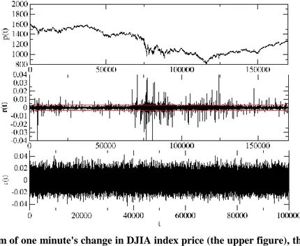
The first financial market evolution model, presented by Louis Bachelier at the beginning of the last century, assumed that the assets price was subject to random walking, and the return had the Gaussian behaviour, so they can be described within a random game [3]. In some financial problems, this model is continued to be used owing to its simplicity, though it does not completely correspond to reality. It is sufficient to look at Figure 2.1 showing the actual financial data (the middle graph) to notice that values occurs in the signals, which have such a large amplitude that practically does not happen in Gaussian distributions. The red line marks the range ±3𝜎 and for the Gaussian variable 99.7% of the values are contained in this range. At first glance, it can be noticed that for the actual data it is quite different. For this particular reason it is generally accepted, and is confirmed by studies, that the distributions of actual financial data have an elongated central distribution part and fat tails. So, these are leptokurtic distributions. The explanation of this phenomenon might be the fact that financial markets experience intermittent problems with liquidity. In the case of high market liquidity, no large price spikes should appear.
Figure 2.1 A diagram of one minute's change in DJIA index price (the upper figure), the returns of this index (the middle figure) and the Gaussian process. The range ±𝟑𝝈 is marked in red.
8
In 1968, Mandelbrot and Van Ness [27] introduced the fractional Brownian motion 𝐵𝐻(𝑡) with the mean value equal to zero and covariance given by the following
formula to describe the financial data: 𝐸[𝐵𝐻(𝑡)𝐵𝐻(𝑠)] = 1
2(|𝑡|2𝐻+ |𝑠|2𝐻−|𝑡 − 𝑠|2𝐻).
(1) Unlike the classic Brownian movement, this is the process with memory, which is dependent on the parameter 𝐻 ∈ (0; 1) and its increments do not need to be independent. In addition, this is a self-affine process, which means that it satisfies the scaling relationship:
𝐵𝐻(𝑐𝑡)~|𝑐|𝐻𝐵𝐻(𝑡). (2)
If 𝐻 > 1/2 we have a persistent time series, in which a positive correlation occurs between successive changes in the series, and the process itself is referred to as a process "with memory". This refers to a long-term memory of the process, which means that the existing change in the series is the resultant of all previous changes, even those very distant, which may only have a fragmentary contribution to the present situations. Moreover, what is happening at present has an effect on distant events in the future. In series of this type, a trend is visible. When 𝐻 < 1/2 the next changes in the series will be correlated negatively, and such a series is called anti-persistent. Consecutive changes between the successive terms of the series are alternating, i.e., if, at a given moment, the series takes on positive values, then it is more likely that it will assume a negative rather than positive value at the next moment. If 𝐻 = 1/2, the process is a random walk and the successive changes in this process will be completely uncorrelated. The parameter 𝐻 defines, therefore, the volatility of the time series. A more detailed description of the 𝐻 is provided in section 4.1.
In the following years, there appeared also geometric and arithmetic Brownian motion models, which relied on the process described by fractional Brownian motion, but which did not have a specific limitation, namely that values assumed by the process might not be negative. They gave better results, though still far from being ideal, just because of the fat tails of the probability distributions of actual data, impossible to be reproduced in the case of the aforementioned processes. Mandelbrot also introduced Levy processes characterized by the probability distribution [7]:
𝐿(𝑥) = 1 𝜋∫ 𝑒−𝛾𝑘 𝛼𝐿cos(𝑘𝑥) 𝑑𝑞 +∞ 0 (3)
9
for the description of the dynamic of financial instrument prices, where 𝛾 > 0 is a scaling factor and the parameter 0 < 𝛼𝐿 ≤ 2 is a stability index. Levi processes have an
infinite variance in the above-mentioned stability range, therefore they do not obey the
Central Limit Theorem 4. The way of overcoming the infinite variance problem in the
context of financial data was the introduction of the Truncated Levy Flights [7], which are given by the following formula:
𝑇𝐿(𝑥) = {𝑐𝐿(𝑥)0 0
−𝑙 ≤ 𝑥 ≤ 𝑙𝑥 > 𝑙 𝑥 > 𝑙
, (4)
where 𝑙 is the length of truncation, 𝑐 is a normalization constant and 𝐿(𝑥), the Levy distribution. Distributions of this type have a finite variance, exponentially decaying tails, and in the central part they are described by the Levy distribution.
As has been previously mentioned, the tails of actual financial data distributions scale themselves following the power law according to the formula:
𝑃(𝑟 > 𝑥)~𝑥−𝛼, (5)
for which 𝛼 ≈ 3. Scaling of this type can be observed in the case of the indices developed share markets, emerging markets and commodity markets, and is called the
inverse cubic law. Distribution of this type are not stable in the Levy sense5 (they have a finite variance), therefore, for sufficiently large time scales, they should converge to the Gaussian distribution in accordance with the CLT. For share markets, the convergence to the Gaussian distribution would be relatively slow with increasing scale [7], though recent studies show [4] that for contemporary markets this convergence is noticeable for scales ∆𝑡 > 1 min.
Another interesting approach to the description of financial markets has been the formalism of nonextensive statistical mechanics proposed by Tsallis in his wok [28]. It is based on the concept of nonextensive entropy which is one of the possible generalizations of Boltzmann-Gibbs entropy. If a given dynamic system is an ergodic system, then this means that its averaged behaviour over time is the same as the behaviour averaged over the set of all available phase space states. This, in turn, means that all microstates are equally likely in the long run. In this sense, the system is
4 In accordance with the CLT, the distribution of a random variable which is a superposition of independent random variables having a finite variance and the expected value equal to, has an asymptotically normal distribution.
5Process 𝑋 is stable, if the sum of independent processes 𝑋
1 and 𝑋2 with a distribution 𝑆, is the process
with the distribution 𝑆: 𝑎𝑋1+ 𝑏𝑋2= 𝑐𝑋 + 𝑑. A feature of stable distributions is that they retain their
statistical properties after summing and scaling. For stable financial time series, minute and hourly returns should have the same variance and mean value.
10
considered in the context of classical Boltzmann-Gibbs thermodynamics which is based on the assumption that all system components are statistically independent and the entropy is given by the formula:
𝑆𝐵𝐺 = −𝑘 ∑ 𝑝𝑖 𝑊
𝑖=1
𝑙𝑛𝑝𝑖.
(6)
The entropy 𝑆𝐵𝐺 for the entire system is the sum of the entropies of the subsystems (it is extensive).
As will be shown in the next sections, the financial market is a system in which all components are interrelated, therefore the use of distributions based on classical thermodynamics is not necessarily the best choice. The approach based on generalized entropy [29]: 𝑆𝑞= 𝑘1 − ∑ 𝑝𝑖 𝑞 𝑊 𝑖=1 𝑞 − 1 (𝑞 ∈ ℛ), (7)
gives better results when applied to empirical data. The parameter q in the formula above defines the statistics, and for 𝑞 = 1 we have simple entropy 𝑆𝐵𝐺. q-Gaussian distributions that maximize the entropy (7) on the assumption that the generalized mean value satisfies the relationship 𝜇𝑞 = ∫ 𝑥 [𝑝(𝑥)]
𝑞
∫[𝑝(𝑥)]𝑞𝑑𝑥𝑑𝑥 and the generalized variance
satisfies the relationship 𝜎𝑞2 = ∫(𝑥 − 𝜇
𝑞)2 [𝑝(𝑥)]
𝑞
∫[𝑝(𝑥)]𝑞𝑑𝑥, are given by the formula:
𝑝𝑞(𝑥) = 𝑁𝑞𝑒𝑞−𝐵𝑞(𝑥−𝜇𝑞)2, (8) where B𝑞 = ((3 − 𝑞)𝜎𝑞2)−1, the q-exponent is defined by the formula 𝑒𝑞𝑥 = [1 + (1 − 𝑞)𝑥]1−𝑞1 while the normalizing factor is:
𝑁𝑞 = { Γ (2(1 − 𝑞)5 − 3𝑞 Γ (2 − 𝑞1 − 𝑞) √1 − 𝑞 𝜋 𝐵𝑞 𝑞 < 1 1 √𝑞 𝑞 = 1 Γ (𝑞 − 1)1 Γ (2(𝑞 − 1))3 − 𝑞 √𝑞 − 1 𝜋 1 < 𝑞 < 3 . (9)
What is important in the case of the q-Gaussian distribution is the fact that it asymptotically takes on the form of a power-law distribution, as follows:
11
𝑝𝑞(𝑥)~𝑥1−𝑞2 , (10)
while if 𝑞 = 1, it assumes the form of a normal Gaussian distribution. For 1 < 𝑞 < 5/3 the sum of q-Gaussians will be convergent to the Gaussian distribution, while for 5/3 < 𝑞 < 3, it will be convergent to the Levy distribution, on account of the Generalized Limit Theorem [30]. It is important, insomuch as using a single parameter 𝑞, it is possible to model a time series being either a monofractal (with the Gaussian distribution) or a multifractal (with the Levy distribution), as will be discussed later in this study.
As shown in reference [31], q-Gaussians can be successfully used for describing the probability distributions of foreign exchange series. Below, some examples of fitting empirical data with these distributions will be shown. For this purpose, the cumulated form of Formula (8) presented in study [31] will be used:
𝑃𝑞±(𝑥) = 𝑁𝑞 ( √𝜋(12 (3 − 𝑞)𝛽 2Γ(𝛽)√𝐵𝛽𝑞 ± (𝑥 − 𝜇𝑞 ) 𝐹 2 1(𝛼, 𝛽; 𝛾; 𝛿). (11)
In the above formula, 𝛼 =12, 𝛽 = 𝑞−11 , 𝛾 =32, 𝛿 = 𝐵𝑞(𝑞 − 1)(𝜇𝑞− 𝑥) 2 , while 𝐹 2 1(𝛼, 𝛽; 𝛾; 𝛿) = ∑ 𝛿 𝑘(𝛼) 𝑘(𝛽)𝑘 𝑘!(𝛾)𝑘 ∞
𝑘 is a hypergeometric Gaussian function.
2.2 Probability distributions of returns
A basic characteristic in examining the statistical properties of financial fluctuations are the probability distributions of returns. These distributions make it possible to construct appropriate theoretical models to describe processes, as well as to look inside them. In the calculations, the logarithmic rate of return, 𝑅 (return), was used, which, for the time series 𝑝(𝑡)representing the value of the signal (price) 𝑝 in time 𝑡, is defined by the following formula:
𝑅 ≡ 𝑅(𝑡, ∆𝑡) = ln(𝑝(𝑡 + ∆𝑡)) − ln(𝑝(𝑡)), (12) where 𝑡 = 1,2, … , 𝑁 is the time instant, and ∆𝑡, the scale under analysis. Then we normalize the returns:
𝑟 ≡ 𝑟(𝑡, ∆𝑡) =𝑅 − 𝑢 𝜈 ,
12
where 𝑣 is the standard deviation of returns in time 𝑇 while 𝑢 is the average value after the time 𝑇. Owing to the normalization, calculations performed for different financial data are comparable. The analysis of fluctuations in returns is best carried out on a log-log scale, because on this scale, power-law relationships take on the form of a straight line, which facilitates the scaling identifications. The distribution of fluctuations is approximately a symmetrical distribution 2.1 2.3, so the absolute values of |𝑟| will be analyzed.
There are a number of studies in the literature concerning the distribution of returns for shares [8; 32], foreign exchanges [31] or commodities [33], however, the statistical analysis presented in this paper, based on high-frequency data in the form of transaction foreign exchange rates, to the author's knowledge, has not been developed yet. For the financial data, a systematic analysis of the statistical properties was started from examining the distributions of the DJIA index returns.
2.2.1 The foreign exchange market (FX)
Forex (FX) is a foreign exchange market, in which various financial institutions, banks, corporations and governments carry out foreign exchange operations. It is an
OTC (Over the Counter) market, where brokers or dealers negotiate currency prices
directly between each other, and there is no central clearing house. This is the largest market in the world with an estimated daily turnover of 5.3 trillion US dollars6. For comparison, the forward exchange market, which is the world's second largest market in terms of turnover, is estimated at less than 440 billion US dollars of daily turnover. Foreign exchange trade takes place round the clock 5 days a week here, excluding weekends, with a huge number of transactions being made; so, this is the most liquid market in the world.
The world's largest foreign exchange broker in 2014 was CITI, whose market share amounted to 16.04%7 and the currency most often traded in 2013 was the American dollar with a market share of 84%8. Movement on the FX has impact on other financial markets, because all other goods are expressed in different currencies, and therefore this market is the world's most important market. From a physicist's point of view, the FX is a complex system with extremely complicated time relationships, as there are many
6http://www.bis.org/press/p130905.htm access on: 24.09.2014
7
http://www.bloomberg.com/news/2014-05-08/deutsche-bank-currency-crown-lost-to-citigroup-on-volatility-1-.html access:24.09.2014 8
13
factors influencing the formation of individual foreign exchange rates. Each of the currency pairs under analysis is characterized by its own dynamics, being dependent of the national economy, central banks (interest rates/inflation) or, as will be demonstrated later on in this study, events taking place in other markets and in different countries.
The performed analysis covered the transaction exchange rates of 9 currency pairs (Figure 2.2) quoted in the period from 17.01.2011 to 21.01.2011, originating from the Deutsche Bank broker, which was the world's second largest broker in 2014:
• GBPUSD-1’157’571 records, • USDJPY-485’169, • GBPJPY – 855’921, • EURUSD-928’925, • EURJPY-1’153’303, • EURGBP-1’359’974, • EURAUD-1’685’455, • AUDUSD-775’698, • AUDJPY-1’204’731.
The data were then converted to the form of equally time-spaced time series with pre-defined intervals of ∆𝑡 : 5-sec. - 86’400 records; 30-sec. - 14’400; 1-min. - 7’200; 2-min. - 3’600; 4-2-min. - 1’800; 10-min. - 720, covering the entire trading day from 00:00 to 24:00 hours.
14
Subjected to analysis were also the so-called triangular relation deviations, which can be described with the following formula:
𝑟∆(𝑡
𝑖, ∆𝑡) = 𝑟𝐴𝐵(𝑡𝑖, ∆𝑡) + 𝑟𝐵𝐶(𝑡𝑖, ∆𝑡)+𝑟𝐶𝐴(𝑡𝑖, ∆𝑡) (14)
and which, assuming the ideal market efficiency 9, should satisfy this equation: 𝑟∆(𝑡
𝑖, ∆𝑡) = 0, (15)
where 𝑟𝐴𝐵 = −𝑟𝐵𝐴. In formula (14), denotes the logarithmic rate of return for the rate of exchange of currency X for currency Y, in time 𝑡𝑖 and on the scale ∆𝑡. Deviations from (15) offer an excellent opportunity for generating profits at no risk, and are referred to as the triangular arbitrage. On contemporary financial markets, such a behaviour of data rates is actually found on very short time scales. Because of this, it is dedicated software programs being at financial institutions' service that close possible arbitrage items by using so-called high frequency trading (HFT)10. Considering the fact that triangular
relation deviations occur at the 6th or a further decimal place, then in order to achieve a measurable profit, it is necessary to invest big money, which essentially precludes the involvement of individual investors.
Using a signal given by formula (14) for analysis, we reduce the number of the system's degrees of freedom, thus going down from three different signal to one. While some exchange rates can be a result of completion of specific investment strategies carried out by traders/institutions, others may be a result of the market movement to eliminate that strategy, or the liquidation of possible arbitrage. When a player buying euros for dollars exchanges dollars for pounds and, for the exchanged pounds, he buys back euros at one time moment, then this transaction will bring in a profit to the player from this transaction, if relationship (15) is greater than zero. The occurrence of such a situation in the market causes the activity of other market participants, as a result of which 𝑟∆(𝑡
𝑖, ∆𝑡) will be convergent to 0.
For examining the triangular relations, the following solid triangles were used:
AUD-EUR-JPY: 𝐴𝑈𝐷𝐸𝑈𝑅∗𝐸𝑈𝑅𝐽𝑃𝑌 ∗𝐴𝑈𝐷𝐽𝑃𝑌 ≠ 0,
AUD-EUR-USD: 𝐴𝑈𝐷𝐸𝑈𝑅∗𝐸𝑈𝑅𝑈𝑆𝐷∗𝑈𝑆𝐷𝐴𝑈𝐷≠ 0,
AUD-USD-JPY: 𝐴𝑈𝐷𝑈𝑆𝐷∗𝑈𝑆𝐷𝐽𝑃𝑌 ∗𝐴𝑈𝐷𝐽𝑃𝑌 ≠ 0,
9
The efficient market hypothesis propounds that, at any time moment, the price of a financial asset fully reflects all the information related to it.
10 HFT is a technique that a large number of transactions to be made automatically using special decision-making algorithms in a very short time (of the order of seconds). www.investopedia.com: access
15
EUR-GBP-JPY: 𝐸𝑈𝑅𝐺𝐵𝑃∗𝐺𝐵𝑃𝐽𝑃𝑌 ∗𝐸𝑈𝑅𝐽𝑃𝑌 ≠ 0,
EUR-GBP-USD: 𝐸𝑈𝑅𝐺𝐵𝑃∗𝐺𝐵𝑃𝑈𝑆𝐷∗𝑈𝑆𝐷𝐸𝑈𝑅≠ 0,
EUR-USD-JPY: 𝐸𝑈𝑅𝑈𝑆𝐷∗𝑈𝑆𝐷𝐽𝑃𝑌 ∗𝐸𝑈𝑅𝐽𝑃𝑌 ≠ 0,
GBP/USD/JPY: 𝐺𝐵𝑃𝑈𝑆𝐷∗𝑈𝑆𝐷𝐽𝑃𝑌 ∗𝐺𝐵𝑃𝐽𝑃𝑌 ≠ 0,
where 𝐴𝑈𝐷𝐸𝑈𝑅,𝐸𝑈𝑅𝐽𝑃𝑌, etc., are the logarithmic rates of return. Figure 2.3 illustrates how the EURUSD exchange rate changes in the period under examination and the returns, r, for ∆𝑡 = 5 𝑠𝑒𝑐. The daily activity of the market is clearly visible in the form of five large clusters. The maximum activity falls, more or less, on the middle of the trading day.
Figure 2.3 The EURUSD exchange rate (top) and the normalized five-second returns calculated for it (bottom).
Figure 2.4 represents the cumulative distributions of returns modules for four selected currencies, though the appearance and behaviour are typical of all the exchange rates examined. Moreover, table 2.1 shows the power-law fitting exponents, using the least squares method, of function given by formula (5) to the distribution tails. It should be expected, similarly as in study [4], that a stronger decline of the distribution tails would be noticed with increasing time scale. However, for the analyzed data, it is difficult to observe such a phenomenon as a rule. For exchange rates based on the Australian Dollar
16
and the GBPJPY currency pair, this is so up to the 2 min. scale, followed by fluctuation on the remaining three scales. For the remaining currency pairs, it is hard to observe any regularity in tail decline; however, it can be assumed that, barring few exceptions, these values are contained in the range between 𝛼 =3 and 𝛼 = 5. This is likely to be influenced by the length of the time series, because of times scales greater than 5 sec., the distribution end scaling region becomes ever shorter and it is difficult to find an exact fit. The analyzed data indicates also that British pound-based exchange rates have the fattest tails, and they do not change very much with increasing time scale. This finding is consistent with previous observations from the period 2004-2008, made in study [31] .
Table 2.1 Power-law exponents for all currency pairs sampled from 5 seconds to 10 minutes.
AUDUSD AUDJPY EURAUD EURGBP EURJPY EURUSD GBPJPY GBPUSD USDJPY
5s 3.99 3.78 4.06 3.76 4.49 4.34 3.51 3.51 4.75 30s 4.83 3.90 4.10 3.91 4.42 4.01 3.62 3.66 3.05 1m 4.91 4.40 4.53 3.43 3.59 4.28 3.81 3.16 3.66 2m 3.67 5.05 3.99 4.09 3.07 3.71 3.44 3.44 3.65 4m 4.18 4.33 4.14 3.66 3.09 3.51 3.13 2.90 3.18 10m 5.03 3.56 3.75 3.79 3.63 3.81 3.44 4.08 3.33
This may also be indicative of the occurrence of correlations in the examined signals, because their convergence to the normal distribution is slower than for uncorrelated signals. As will be demonstrated later on in this study, these are nonlinear correlations being behind the fractal nature of the examined processes.
17
Figure 2.4 Cumulative distributions of currency returns, determined for time scales from 5 sec. to 10 min.
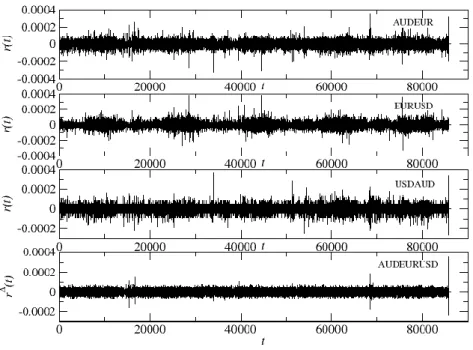
The situation is slightly different for the distributions of triangular relation deviations. Already at the returns level, a difference between 𝑟∆ and its component signals can be
seen. While the fluctuation magnitudes are the same, the structure of the series 𝑟∆ itself
is more uniform, with a small number of large-amplitude events. This is illustrated in Figure 2.5 for the AUD-EUR-USD pair.
18
Figure 2.5 The times series of three exchange rates making up the AUD-USD-EUR triangle and the triangle itself (the series at the very bottom).
In contrast to the returns distributions, starting from the 5-second scale, the characteristic inverse cubic scaling law was not observed. All obtained scaling exponents assume values 𝛼 > 3, and the distribution tails are practically of the Gaussian type. The only exception is the EUR-GBP-JPY triangle, where, except for the 2-minute scale, the scaling exponents lie in the range of 𝛼 ∈ (3; 4).
19
Figure 2.6 The cumulative distribution of triangular relation deviation returns, determined for the time scale from 5 sec. to 10 min. Panel a) shows AUD-EUR-JPY triangular relation deviations, b) EUR-USD-JPY, c) EUR-GBP-USD, d) AUD-USD-JPY, e) EUR-GBP-JPY.
A complete list of power exponents fitted to the distributions of triangular relation deviations is given in Table 2.2 .
Table 2.2 Power exponents for all triangular relation deviations sampled from 5 sec. to 10 min.
AUD-JPY-USD AUD-EUR-USD AUD-EUR-JPY GBP-USD-JPY EUR-GBP-USD EUR-GBP-JPY EUR-USD-JPY 5s 5.77 4.36 7.28 7.44 8.71 4.07 6.66 30s 5.90 5.82 7.35 8.40 6.75 3.74 7.49 1m 5.67 5.20 8.14 5.53 8.12 3.91 6.91 2m 5.74 5.22 6.61 6.73 5.60 4.98 6.89 4m 7.01 4.31 7.63 7.11 6.60 3.90 5.44 10m 5.66 4.58 5.39 6.63 4.46 3.21 5.61
As has been mentioned above, q-Gaussians prove themselves very well in describing real financial data. For this reason, their usefulness for the description of Forex market data was verified. Due to the length of the series, the distributions were fitted only to
5-20
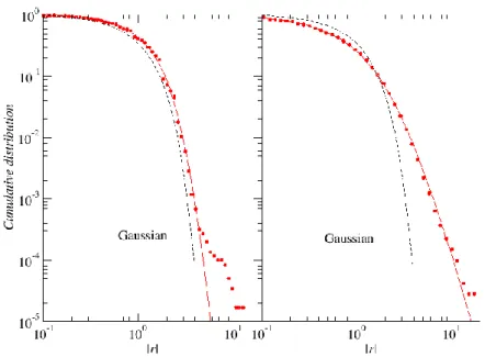
second time series. Figure 2.7 shows a cumulative distribution for the AUD-EUR-USD triangle and the AUDUSD exchange rate with the q-Gaussian function fitted.
Figure 2.7 The distribution of fluctuations in 5-second AUD-EUR-USD triangular relation deviations (the left-had panel) and the AUDEUR exchange rate (the right-hand panel) along with the q-Gaussian function fitted to the distribution tail (the solid line). The dashed line indicates the Gaussian distribution.
These results are representative of all the examined triangles and currency pairs. It is clearly seen that, for the exchange rates, the distribution tails coincide very well with the value of the fitted function. In the case of the triangles, these distributions fairly well coincide with one another in the central part, whereas the tails are modelled not very accurately, and the empirical data are overrepresented with respect to the fitted
distribution, more for the signal 𝑟∆ than for the returns themselves. For EURAUD 𝑞 =
1.44, which, according to formulae (5) and (10), means that the distribution tail scales itself approximately with the exponent 𝛼~4.5.
2.2.2 DJIA
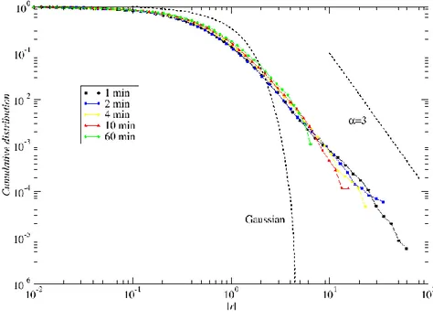
In a similar way, 29 DJIA index companies and the index formed from those companies were analyzed. As has been shown in study [34], the index and its individual components are processes subject to the same probability distribution. The quotations covered the period 02.01.2008 –29.07.2011 and these were one-minute data. The index was made in a manner specific to this type of data, i.e. the share prices at a given time moment were added together, and then the returns were calculated from that signal.
21
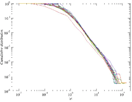
Records formed through so-called share splits 11 likely to cause artificial fluctuations in data analysis, were removed from the time series. Figure 2.8 below represents the cumulative distributions of the one-minute normalized returns of all companies.
Figure 2.8 The normalized cumulative distributions of 1-minute returns of 29 DJIA index companies.
For the entire set, a very similar behaviour and power-law tail scaling can be noticed. The power-law behaviour of the tails is exhibited by distributions that have a finite variance and are either unstable distributions or stable distributions with the scaling exponent assuming values 𝛼 ≤ 2. Table 2.4 summarizes all power exponents fitted to the distribution tails.
Table 2.3 The power exponents of power-law distribution fitting to the 1-minute cumulative distributions of DJIA index companies.
AA 2.52 CSCO 2.51 INTC 2.67 MMM 2.55 T 2.8 AIG 2.15 CVX 2.47 JNJ 2.59 MRK 2.45 UTX 2.52 AXP 2.62 DD 2.56 JPM 2.47 MSFT 2.53 VZ 2.48 BAC 2.22 GE 2.53 KFT 2.37 PFE 2.49 WMT 2.62 BA 2.59 HD 2.57 KO 2.67 PG 2.49 XOM 2.64 CAT 2.53 IBM 2.44 MCD 2.64 TRV 2.67
Tail scaling along with the increase in the index time scale is illustrated in Figure 2.9. As can be noticed, the exponents take on values 𝛼~2.5 and lie beyond the stable Lèvy
11 A share split is a reduction in the value of a given share, with the current level of the company's share capital being maintained. Some companies, wishing to maintain the prices of their shares in a range chosen by them, either emit new shares or split the share price, while retaining the share capital.
22
region and, with increasing times scale, they come ever closer to the Gaussian distribution, which is consistent with the Central Limit Theorem.
Figure 2.9 The cumulative distribution of the DJIA index for five time scales.
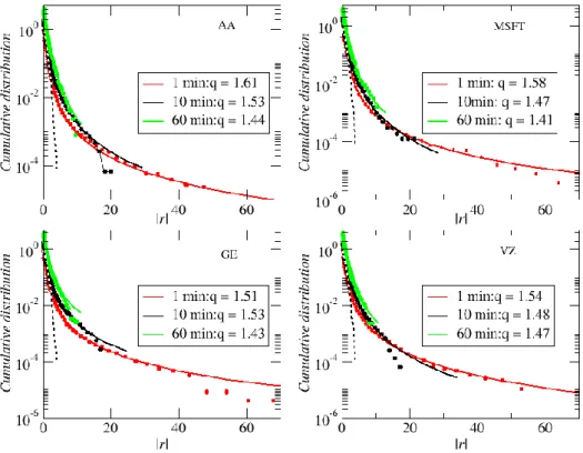
Similarly as for the FX market, an attempt was made to fit the q-Gaussians to the distribution of empirical data depending on the parameter q. As the representative set, four companies from different industries were chosen: AA – American Airlines (the aircraft industry), GE – General Electric (conglomerate), MSFT – Microsoft (IT), VZ – Verizon (telecommunications). The fitting was prepared for three time scales ∆𝑡 ∈ {1,10,60} minutes, and its result is shown in Figure 2.10. The obtained result seems to be very good, as the central part of the distribution and a considerable part of its tail coincide perfectly with the theoretical values. Only very rare events occurring at the very end of the distribution diverge slightly. In all cases, with the increase in the time scale, the values of parameter q decrease. This could have been expected from the asymptotic form of the q-Gaussian (10) and the previously observed fact of the convergence of the distribution tails to the Gaussian distribution with the increase in ∆𝑡.
23
Figure 2.10 The cumulative distributions of the returns of four companies with the q-Gaussian function fitted to the distribution tail.
2.3 Autocorrelations and time cross-correlations
Cross-correlations occurring in financial data provide an extremely important element of the analysis of their dynamics. They are part of stylized facts which, in this case, make the function of autocorrelation of the financial time series drop to zero after several minutes [8; 35], while for the volatility (the module of the returns under examination) this function remains positive over a considerable period of several weeks [36]. The autocorrelation (self-correlation) function 𝜌𝑥(𝜏) for function 𝑓(𝑡) and shift 𝜏 is defined as follows:
𝜌𝑥(𝜏) = 〈𝑓(𝑡 + 𝜏)𝑓(𝑡)〉. (16)
With the use of this function, we can determine the effect of the current signal value on the signal value in the future. The function may assume either positive values (when the changes between analyzed values in the series follow one another in the same direction) or negative values (the changes between series values follow one another in the opposite directions) and the maximum falls on the zero-shift point. For random signals, the function value falls immediately to zero. This function lends itself perfectly to the examination of linear relationships in an examined series.
24
The next stage in the investigation of FX market dynamics will be examining the interrelation between financial data. This is a very important analysis that is widely used in finances, because it leads to the optimization of the investment portfolio and assists in managing the risk. In the analysis of time series and processing signals, the cross-correlation (intercross-correlation) between two series is described by normalized covariance that means the degree in which the two series follow one another, assuming that one of these series is shifted by 𝜏 relative to the other. For two series 𝑋𝑡 and 𝑌𝑡 with a length T, this relationship is defined by a cross correlation function which is given by this formula:
𝜌𝑥𝑦(𝜏) =∑𝑇𝑡=1(𝑋(𝑡) − 𝜇𝑋)(𝑌(𝑡 + 𝜏) − 𝜇𝑌)
𝜎𝑋𝜎𝑌 ,
(17) where 𝜎𝑋 and 𝜎𝑌 is the standard deviation of the respective series, while 𝜏 is the shift of the series 𝑌 relative to 𝑋. In the case, where 𝜌𝑥𝑦(𝜏 = 0), this is the Pearson correlation coefficient that assumes values in the interval −1 ≤ 𝜌𝑥𝑦 ≤ 1. In the case, when 𝜌𝑥𝑦 =
1, we have a perfect correlation between the signal, where 𝜌𝑥𝑦= −1 means
anti-correlation and 𝜌𝑥𝑦 = 0 lack of correlation between the signals. Using 𝜌𝑥𝑦, the level of linear relationship between the signals 𝑋𝑡 and 𝑌𝑡 is determined. From this point on in this study, the terms cross-correlation and intercorrelation will be used interchangeably. Returns, as well as their modules, were used for analysis in view of the fact that the autocorrelation of volatility may exhibit a different nature.
2.3.1 DJIA
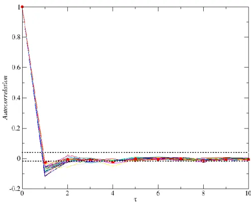
The results obtained for the returns of the DJIA index companies discussed in the previous section are shown in Figure 2.11. They clearly indicate that no long-range correlations occur in financial signals, and only for 𝜏 = 1 min. can we speak of a weak anti-correlation of the examined time series. A possible cause of this phenomenon is the occurrence of zeros in the values of the returns on short time scales, being comparable to, or shorter than the frequency of making transactions. Negative autocorrelation is therefore a computational artefact. The behaviour of the entire index is similar, except that in the first minute the autocorrelation level is less negative compared to all component companies and takes on a value close to the noise value. Looking at the process governing the share price from this perspective, one might arrive at the conclusion that it is of the Brownian type (has no memory).
25
Figure 2.11 Autocorrelation function determined for 1-minute returns of 29 DJIA index companies. The index autocorrelation function is marked with the red line. The dashed lines denote the noise level.
In addition to examining the autocorrelation of the returns, their modules, i.e.
volatility, was subjected to analysis. This quantity directly takes advantage of the
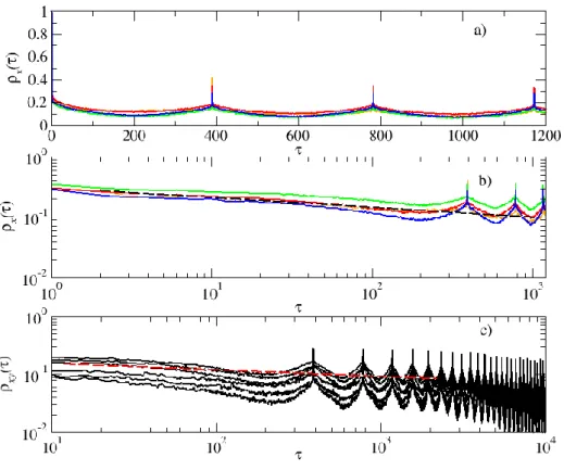
amount of information coming in to the stock exchange. Panel a) in Figure 2.12 represents this value on a linear scale for four companies: AIG, GE, MSFT and CSCO. We can clearly see a daily trend in the form of the regularity of a function, in which characteristic peaks occur exactly every 390 minutes. Panel b) in the above-mentioned figure shows the same data, presented on the log-log scale, along with a power-law function fitted to them. It can be seen that the autocorrelation function of volatility is long-range in character, in contrast to the examined returns. The power-law function fitted to the empirical data (given by formula (5)) has an exponent 𝛼 = 0.16 and seems to adequately describe the character of the fading of correlation in the signal. The same behaviour is visible in Panel c), which shows the intercorrelation function determined for those companies and fitted to the data with a power-law function with power exponent 𝛼 = 0.11.
26
Figure 2.12 The autocorrelation of volatility. Panels a) and b) show the function of autocorrelation of the volatility of four companies. The company AIG is marked in orange colour, GE in red, CSCO in green and MSFT in blue. Panel c) represents the cross-correlation determined among these companies. The dashed line denotes the power-law fit. A daily trend with characteristic peaks every 390 minutes (1 trading day) is clearly visible.
Using formula (17), the Pearson coefficient among all companies returns has been determined, which yields 406 possible combinations. All of the examined companies are positively correlated with one another. Two thresholds of correlation values are very well visible, i.e. at 𝜌𝑥𝑦(0) ≈ 0.4 and 𝜌𝑥𝑦(0) ≈ 0.5, in the vicinity of which more than
half of the obtained values lie. This is indicative of a moderate strength of those correlations. In the case of 41 combinations of companies, there is no cross-correlation between signals, and two of them are correlated with each other at a level of 𝜌𝑥𝑦(0) =
0.7. The mean value of cross-correlation in the examined set is 𝜌̅̅̅̅̅̅̅̅̅ = 0.35 . When 𝑥𝑦(0)
comparing the cross-correlation of companies from different sectors in Table 2.4, it can be noticed that its mean value is the greatest for Materials sector companies, while the least for Services sector companies.
Table 2.4 The mean value of returns cross-correlation 𝝆𝒙𝒚(𝟎), given by sectors.
27 Consumer Goods 𝜌̅̅̅̅̅̅̅̅̅ ≈ 0.36 ± 0.02 𝑥𝑦(0) Financial 𝜌̅̅̅̅̅̅̅̅̅ ≈ 0.32 ± 0.07 𝑥𝑦(0) Healthcare 𝜌̅̅̅̅̅̅̅̅̅𝑥𝑦(0) ≈ 0.34 ± 0.02 Industrial Goods 𝜌̅̅̅̅̅̅̅̅̅ ≈ 0.39 ± 0.01 𝑥𝑦(0) Services 𝜌̅̅̅̅̅̅̅̅̅ ≈ 0.28 ± 0.06 𝑥𝑦(0) Technology 𝜌̅̅̅̅̅̅̅̅̅ ≈ 0.35 ± 0.08 𝑥𝑦(0) 2.3.2 FX market
A similar analysis was made on data from the foreign exchange market, where the strength of correlation between each of the 9 currency pairs was determined. Figure 2.13 represents autocorrelation functions, as dependent on the delay 𝜏, for all currency pairs (the top diagram), as well as triangular relation deviations (the bottom diagram). Just like for financial markets, for FX data this function will assume values at the zero level, practically from 𝜏 = 2. Similarly as in study [31], a characteristic feature of almost all examined currency pairs is the existence of a correlation low of negative correlations for 𝜏 = 1, being indicative of an (apparent) anti-persistence of the series for short time scales. The only currency pair that has no low for 𝜏 = 1 is GPBUSD, which, apart from the EURUSD pair (the minimum low), is the most frequently traded currency pair. Therefore, the series of their returns have the fewest zeros, and it is the presence of zeros that determines whether the occurring persistence is apparent or not. If price-changing transactions occur rarely, then returns different from zero seldom happen in the signal, as isolated peaks surrounded by zeros on both sides. That is, effectively for the algorithm, the large (real) rate of return is followed by a small one (or zero). This resembles exactly persistence, but is not it. Therefore, the negative anti-correlation determined for the FX data is a computational artefact.
28
Figure 2.13 The autocorrelation function of 5-second returns corresponding to all currency pairs (the top panel) and triangular relation deviations (the bottom panel).
This implies that the process memory is very short, which is characteristic of Brownian processes.
The volatility autocorrelation functions can be seen in Figures 2.14 and 2.15.
Figure 2.14 The top panel: volatility autocorrelation of 5-second data. Peaks constituting a daily trend are clearly visible. The bottom panel: the volatility of triangular relation deviations for 5-second data.
29
Figure 2.15 The volatility autocorrelation function on the log-log scale of 5-second time series corresponding to all currency pairs (the top panel) and triangular relation deviations (the bottom panel).
When comparing the volatility with the returns it can be seen that the autocorrelation has a long decay time. In approximation, this is a power-law relationship 𝑐(𝜏)~𝑥−𝛼, and the power exponent assumes the values 𝛼 = 0.32 and 𝛼 = 0.15, respectively, for returns and the triangular relation deviations.
Using the converse exchange rates (𝐸𝑈𝑅
𝑈𝑆𝐷 = ( 𝑈𝑆𝐷 𝐸𝑈𝑅)
−1
), it was possible to examine 24 currency pairs "in the triangle" and 12 currency pairs "beyond the triangle" for cross-correlations. A complete list of combinations is provided in Table 2.5.
Table 2.5 24 exchange rate pairs "in the triangle" (black colour) and 12 exchange rate pairs "beyond the triangle" (red colour).
AUDJPY/EURAUD AUDJPY/JPYUSD AUDJPY/USDAUD
AUDUSD/USDEUR AUDUSD/USDJPY EURAUD/GBPEUR
EURAUD/AUDUSD EURAUD/USDEUR AUDJPY/GBPJPY EURJPY/AUDEUR EURJPY/JPYAUD GBPUSD/USDJPY GBPUSD/EURGBP GBPUSD/JPYGBP GBPUSD/USDEUR GBPJPY/JPYEUR GBPJPY/JPYUSD GBPJPY/EURGBP EURJPY/USDEUR EURJPY/JPYUSD EURGBP/JPYEUR
EURUSD/GBPEUR EURUSD/USDJPY AUDUSD/USDGBP
AUDJPY/EURGBP AUDJPY/GBPUSD AUDUSD/EURGBP
EURJPY/GBPUSD EURJPY/AUDUSD EURUSD/AUDJPY GBPUSD/EURAUD GBPJPY/AUDUSD EURAUD/GBPJPY
30
EURAUD/USDJPY EURGBP/USDJPY EURUSD/GBPJPY
The employed denotation "currencies inside the triangle" means a simplified version of triangular arbitrage, where one single currency will occur between the examined exchange rates. This name will be used later on in this study. In the case of exchange rates "outside the triangle" we have four independent currencies. Moreover, it can be expected that the condition 𝐴𝑈𝐷𝐽𝑃𝑌 ∗𝐴𝑈𝐷𝐸𝑈𝑅= 𝐸𝑈𝑅𝐽𝑃𝑌 will be satisfied for currencies inside the triangle, which enables, using two different exchange rates 𝐴𝑈𝐷𝐽𝑃𝑌 and 𝐴𝑈𝐷𝐸𝑈𝑅 having a common currency 𝐴𝑈𝐷, the determination of the exchange cross-rate 𝐸𝑈𝑅𝐽𝑃𝑌. For currencies outside the triangle, as in the case of 𝐴𝑈𝐷𝐽𝑃𝑌 ∗𝐸𝑈𝑅𝐺𝐵𝑃, it is not possible to calculate the exchange cross-rate, because there is no common currency between the exchange rates.
The relation between exchange rates was examined using formula (17). Except for the AUDJPY/GBPJPY pair, all currencies inside the triangle are negatively correlated, while those outside the triangle, correlated positively (except for the pairs EURAUD/USDJPY and EURGBP/USDJPY). The most negatively correlated is the EURUSD/GBPEUR pair with a correlation value of 𝜌𝑥𝑦(0) = −0.63, AUDJPY/GBPJPY is positively correlated with 𝜌𝑥𝑦(0) = 0.37, while the GBPJPY/AUDUSD pair is almost uncorrelated, with 𝜌𝑥𝑦(0) = 0.06 (the noise level is 0.01). All the results for 𝜌𝑥𝑦(0) are shown in the inner panel in Figure 2.16. The mean value of the correlation coefficient for the pairs inside the triangle is 𝜌̅̅̅̅̅̅̅̅̅ = −0.36, 𝑥𝑦(0)
which means a negative intercorrelation, while for the pairs outside the triangle it is 𝜌𝑥𝑦
̅̅̅̅̅(0) = 0.19, which would suggest virtually no or very little intercorrelation. This value is disturbed by the aforementioned pairs: EURAUD/USDJPY with the coefficient 𝜌𝑥𝑦
̅̅̅̅̅(0) = −0.08 and EURGBP/USDJPY with 𝜌̅̅̅̅̅(0) = −0.13. The EURUSD pair is 𝑥𝑦 the one which is strongest linked with the remaining exchange rates and has the mean correlation coefficient equal to 𝜌̅̅̅̅̅̅̅̅̅ = −0.31. This result could have been expected, 𝑥𝑦(0) as this pair is the world's most often traded currency pair with a 25% market share12. In turn, an exchange rate least connected with other exchange rates is the AUDJPY with
12
31 𝜌𝑥𝑦(0)
̅̅̅̅̅̅̅̅̅ = −0.13 being, at the same time, a pair with the smallest quota market share (approx. 0.5 %) among the most popular exchange rates.
In the next step, the cross-correlation between the volatility of all currency pairs from Table 2.5 was examined. This is represented in Figure 2.16 where the currencies inside the triangle are shown in black, while the currencies outside the triangle, in red.
Figure 2.16 The cross-correlation function determined for the volatility of 5-second time series. The currencies inside the triangle are indicated with black colour, while the currencies outside the triangle, with red. The dashed line denotes the noise level. The inset shows the Pearson correlation coefficient 𝝆𝒙𝒚(𝟎), determined for the returns.
At the volatility level, all the examined exchanges rates are cross-correlated for events distant as much as by 5 ∗ 103 (which gives almost 7 trading hours). For a delay of about
50 seconds, a slightly lower level of cross-correlation can be observed in the currencies outside the triangle, compared to the currencies inside the triangle. In the inset, the cross-correlation level for the returns is also indicated. Cross-correlation clustering on the negative value side for currencies inside the triangle is clearly seen. The only exception is the AUDJPY/GBPJPY currency pair.
Figure 2.17 illustrates cross-correlations between triangular relation deviations. Deviation pairs, for which 2 common currencies exist, such as AUD-USD-JPY/AUD-USD-EUR (with the common currencies AUD and USD), are marked in red colour, while those that have one common currency, e.g. AUD-USD-JPY/GBP-JPY-EUR (the
32
common currency being JPY), are marked in black. It is clearly visible that, in the case of two common currencies between deviations, there is a cross-correlation for a delay of up to 𝜏 = 3 (equal to 15 sec.), thereupon it assumes the level of two uncorrelated noises. In the case of one common currency, the cross-correlation between two series is
immediately zero. This results from the fact that for currency triangle pairs, two information transferring currencies are needed in order to be able to determine the cross-correlation between them.
Figure 2.17 The function of cross-correlation between triangular relation deviations. Correlations between triangles having 2 common currencies are marked in red colour.
33
3 Fractal and multifractal formalism
In the classical Euclidean geometry, we generally deal with regular objects, that are the ones free from roughness (such as curves, polygon sides, spheres or polyhedron walls). As can be easily noticed, the world around us is not so regular and simple in description. The attempt to describe the shape of some real objects (e.g. clouds) using traditional geometry is sometimes a very tedious, if not impossible job. In the 1970s, Benoit Mandelbrot made some groundbreaking discoveries in the study of irregular objects and created fractal geometry [37; 38]. From that moment, fractals have changed the way we view the world. The word 'fractal' itself is derived from Latin and means 'fractional' or 'broken'. When examining financial data charts, Mandelbrot noticed that they are similar to each other in different time scales. This is a feature that is characteristic of fractals and is called self-similarity. An object having this feature is similar to itself regardless of the scale, looking the same when observed either from close up or from a distance. Taking a part of an object and respectively scaling it, we will get an object similar to the whole. Using fractal geometry, we can examine systems, from the complex and irregular structure of which, an ordered and hierarchical picture will emerge. Fractals are present almost everywhere. The shapes of a snow flake, shoreline, trees, human lungs or broccoli – these are just a few examples of natural, random fractals, in which self-similarity is statistical in character. One flake may differ in details from the other, but in terms of general characteristics, they are the same. And it is this type of systems that can be most fully described using fractal geometry. Apart from them, there are plenty of mathematical (deterministic) fractals generated by recurrent formulas, which, unlike natural fractals, make up ideal structures. At each iteration, scaling takes place while preserving the characteristic scale, which is not a rule for random fractals. Very commonly, random fractals are used in video games and computer graphics, where, with the help of simple mathematical rules, complex structures are created, including most often some landscape elements, such as trees or mountains, at a much lower computing cost. Examples of such fractals are shown in Figure 3.1.
34
Figure 3.1 Examples of simple mathematical fractals (on the left). The second top structure is a Koch curve, while the first bottom one, a Sierpinski triangle. On the right, there are examples of natural fractals.
Also the time series of financial data have a fractal nature. Looking at the time series of data recorded every second or every minute, it is very difficult to distinguish which series is on what scale (Figure 3.2).
Figure 3.2 Self-similarity of a time series (EUR/USD).
Moreover, the record of share price variations (assuming its continuity) is not one-dimensional (it is not an ordinary curve) or two-one-dimensional (its surface has a zero area), which, according to the definition below, is sufficient to refer it as a fractal. In addition, unlike classic fractal forms, which are spatially self-similar, time series are self-similar with respect to time.
35
There is no single definition of the fractal. One of the definitions says that the fractal is a set that exhibits a self-similarity property, at least in an approximate sense, if not exactly. According to another definition, fractals are objects having a non-trivial structure, which cannot be described using the Euclidean geometry. Or, the fractal is an object whose dimension is not an integer.
We assume that the set 𝐹 is called fractal, if it shows the following features [39]: 1) 𝐹 has a structure such, that its details can be seen on an arbitrarily small scale; 2) 𝐹 is too irregular to be described using traditional geometry;
3) 𝐹 is self-similar (in a statistical sense);
4) fractal dimension of 𝐹 is usually greater than its topological dimension;
5) in the case of mathematical fractals, it is defined simply, most fully in the form of a recurrent procedure.
Below, basic fractal geometry concepts necessary for the description of fractals will be presented.
3.1 General properties of fractal sets
Fractals are scale free objects, i.e. they do not have a single, distinguished scale. They exhibit so complex structure that no direct and accurate measurement of their length, surface area or volume is possible. During the measurement of these values, it is normally indicated how fast they increase, because when made with increasingly great accuracy, the measurement will lead to divergent results. It should be noted that not every self-similar object is a fractal. Objects not being fractals include, e.g., an interval, a square or a cube. If the linear dimensions of those objects are scaled by an arbitrary number, then their respective surface area and volume will be changed proportionally. In the case of fractals, there is no such proportionality.
Scaling is, therefore, a superposition of several transformations in Euclidean geometry. The transformation 𝑆: ℝ𝑛 → ℝ𝑛 is called isometric, if it retains the distance,
that is |𝑆(𝑥) − 𝑆(𝑦)| = |𝑥 − 𝑦| for every 𝑥, 𝑦 ∈ ℝ𝑛. An example of isometric
transformation is translation, or the parallel shift S(x) by a vector a: 𝑆(𝑥) = 𝑥 + 𝑎,
rotation about a point 𝑎, |𝑆(𝑥) − 𝑎| = |𝑥 − 𝑎| and reflection. Similarity transformation
by a value c is a transformation, where the relationship |𝑆(𝑥) − 𝑆(𝑦)| = 𝑐|𝑥 − 𝑦| occurs for every 𝑐 > 0 and 𝑥, 𝑦 ∈ ℝ𝑛, whereby a geometric figure subjected to this transformation turns into the identical figure, but with all its dimensions multiplied by
36
the value c. This is an isotropic transformation, i.e. the transformed object is scaled by the same value in all directions.
A special case of self-similarity is self-affinity. The affine transformation 𝑆 is a transformation in the form of:
𝑆(𝑥) = 𝑇(𝑥) + 𝑎, (18)
where 𝑎 is a point in ℝ𝑛 while 𝑇 is singular linear transformation. A transformation 𝑇 is
non-singular, if 𝑇(𝑥) = 0 ⟺ 𝑥 = 0 and 𝑇 if the following relationship occurs:
𝑇(𝑥 + 𝑦) = 𝑇(𝑥) + 𝑇(𝑦) i 𝑇(𝜆𝑥) = 𝜆𝑇(𝑥), (19) where 𝑥, 𝑦 ∈ ℝ and 𝜆 ∈ ℝ.
Affine transformation can be understood as a superposition of the operations of scaling, translation, rotation and reflection, not necessarily by the same value in all directions. So, this is an anisotropic transformation, in which scaling depends on the orientation in space. An example of affine transformation is shown in Figure 3.3 below.
Figure 3.3 A schematic diagram of affine transformation.
Self-affine are the time series of the returns (Figure 3.2), and for the description of the degree of irregularity of function 𝑓(𝑥) that can represent such a time series, the Hurst exponent 𝐻 is used. In the case, where 𝑓(𝑥) is self-affine, it satisfies the following relationships:
𝑓(𝑥) ≅ 𝜆𝐻𝑓(𝜆𝑥). (20)
It follows from formula (20) that for 𝐻 = 1, 𝑓(𝑥) is self-similar. When the exponent 𝐻 is dependent on time t, then the Hölder exponent (function) [40] is used to define the pointwise scaling. A function 𝑓 is called the Hölder function with an exponent ℎ, if the following relationship is satisfied: