A WAY OF SIMULATION TRANSPORT PROCESSES
AND DISTRUBANCES IN SUPPLY CHAIN
Patrycja Hoffa-Dąbrowska* and Paweł Pawlewski**
Faculty of Engineering Management, Poznan Univesity of Technology, Poznan 60-965, Strzelecka 11, Poland,
* Email: hoffa.patrycja@gmail.com ** Email: pawel.pawlewski@put.poznan.pl
Abstract The paper presents a description of how to model the supply chain using simulation software. In order to make the best representation of reality, not only the route and the lorry’s speed are taken into account, but also the presence of various types of disturbances, like the occurrence of severe weather conditions or the inclusion of the driver's breaks, according to the applicable regulations. The purpose of this article is to demonstrate how to model the disturbance and to present benefits of using of simulation programs to plan a route of transport.
Paper type: Research Paper Published online: 30 April 2016
Vol. 6, No. 2, pp. 141-153
DOI: 10.21008/j.2083-4950.2016.6.2.4
ISSN 2083-4942 (Print) ISSN 2083-4950 (Online)
© 2016 Poznan University of Technology. All rights reserved.
1. INTRODUCTION
Paper presents author's work about how can we model a supply chain including different disturbances occurring in transport processes. Because of range aspects including in supply chain, they concentrate on transport area. Networks in supply chain can be modeled in different way, like by using Petri net, or algorithm Dijks-tra and /Floyd-Warshall algorithms or by using simulation. In this article authors want to show using of simulation to model supply chain. Based on case study they show how we can model networks in supply chain and how can we model disturb-ances. One of them is described in detail. In presented case study, the route for reali-zation transport order is defined, including different variables, as: a vehicle speed and different disturbances, as: severe weather conditions and breaks in driver works. This model is created by using a modern software FlexSim, that allows build models of various degrees of complexity (https://www.flexsim.com). To model disturb-ances, authors integrate Discrete Event Simulation (DES) with an Agent Based Simulation approach (ABS). Disturbance is represented by own created object, which has some intelligence, which has been given by modeler.
The main aim of this article is to present a simulation model of transport route for presented using simulation software to manage of some area of supply chain. To present processes in the best reality way, authors model route with some assump-tions, like vehicle’s speed. Besides, they include disturbances in this route. In this case they consider two disruptions – bad weather conditions and breaks in driver working time. Authors describe in detail how one of this disturbance is created in simulation model, not only in theoretical. Thanks to using simulation to model transport task, observation and analyze of dependences and behavior is possible. Moreover, making different experiments, user can see what will change, and how it will affect to whole process.
2. THE SUPPLY CHAIN ISSUE AND ASPECT OF OCCURRENCE
DISTURBANCES IN SUPPLY CHAIN
2.1. The complexity of the supply chain issue
The first thought when we hear "supply chain", is an association with transpor-tation process of products from point A to point B. But the issue is more complexi-ty. Of course, the main role of the supply chain is a transportation of products from one point to the other, but we have to consider many other aspects, such as: ensur-ing adequate quality services at the lowest cost, findensur-ing the best mode of transport, the management of different entities involved in whole process.
At present, supply chains are dispersed systems (Caddy & Helou 2007); (Wie-land & Wallenburg 2011). What makes, that the next problem is how to manage links and the structure of the whole chain in order to achieve the best results (in strategical and financial dimension).
Therefore, people pay more attention to modeling the supply chains and man-agement of them by using various computer programs. The network can be de-scribed and modeled in few ways – the most know are:
• modeled transport routes by using different type of network, for example Petri net (Skorupski, 2011);
• by using algorithm like Dijkstra and /Floyd-Warshall algorithms (Chen et al. 2009);
• in mathematical description (Wilhelm & Hollunder 2007); • and by using simulation software (http://www.llamasoft.com/).
For the purposes of modeling the processes in the supply chain two methods are used: Discrete-Event Simulations (DES) and Agent-Based Simulation (ABS). First method is a good option when we deal with well-known processes, for which the situations of uncertainty are defined using statistical distributions. DES models are characterized by the process approach – they focuses on modeling the system in detail, not on the independent units (Cassandras & Lafortune 2008). Second meth-od, focus on individual elements and their behaviors (Kim & Robertazzi 2006). Ref-fering to the supply chain – the individual chain participants (companies, manufac-turers, wholesalers and retailers) can be treated as agents who have their own goals and skills, and their common goal is to produce and deliver a product to a specific customer (http://www.anylogic.com). Agent-Based Simulation is discussed in more detail in (Kim & Robertazzi 2006); (Macal & North 2013). There are also numerous articles dedicated to agent modeling and multi-agent modeling in the transport and supply chains (Balbo & Pinson 2005); (Bocewicz et al. 2013).
2.2. The aspect of occurrence the disturbances in supply chain
Analysing transportation process, it is important to see broader range of this ac-tivity, not only the moving of goods. As in any other process, we should take into account the presence of various types of interference in the realization of activities. In literature, we can find many articles about issue of the transport of hazardous materials and the associated with this transport risks (Gheorghe et al. 2004); (Mar-seguerra et al. 2003); (Tixier et al. 2006). Other popular aspect are car accidents (Orlandelli & Vestrucci 2004).
Authors it their works, focus on transport area in supply chain, and aspects of realization transport task in time. That’s way they decided to distinguish various disturbances in this area, and try to determine how they affect to realization of whole process and time of it (Hoffa & Pawlewski 2014b). Authors distinguished such disturbances in transport operations (Hoffa & Pawlewski 2014a): related with
means of transport (like the failure of vehicle); related with the route (like: the traf-fic congestion, the road accident, weather conditions, the fee payment in Toll Col-lection Point); resulting from the fault of the sender and receiver (like: no enough free ramps for loading/unloading); related with the driver (like: the driver working time); and other.
3. PROBLEM DEFINITION
During the analysis of the literature about various disturbances in transport, au-thors noticed that a little number of articles about way of modeling of these dis-turbances are exists. Therefore, they decided to concentrate on the modeling the disturbances with the determination of the influence of them on the transport process, on time of transport.
Authors present mathematical description of the supply system model. Next, they show simulation model of the supply chain.
3.1. The supply system model – mathematical description
Authors present general description of model of a supply system (Fig.1).Fig. 1 The supply system model
A supply system model (Fig.1) is defined as: Where:
P - a transport route, defined as a sequence of:
- intermediate point, where disturbances are considered, - the number of intermediate points,
- a starting point (load point), - an unload point.
Intermediate points – are locations where interference may occur in the delivery.
Disturbances may affect to the delivery time.
- a sequence of distances between intermediate points:
(3) - the distance between the point and point ,
- sequence of transit times between intermediate points:
(4) - a travel time from the point to counted in contractual units of time [c.u.t.], . The travel time is defined as a continuous random variable, for which it is known probability density distribution
. The probability of density distribution is dependent on the type of disturbance.
For the supply system modeled by the SD (1), in addition total time of delivery is defined .
(5) where:
- a time of loading of i-th pallets [c.u.t.], - a number of pallets.
Total time of realization the delivery determine date of unloading : (6) where:
- date of loading [c.u.t], , - expected date of unloading, .
For presented system, is searched answer for question: Is there a time of starting the loading , which ensures, with the specified probability Pd, ending the
deliv-ery at defined interval ?
for ,
3.2. The simulation model of supply chain - general information
In order to show how can we use simulation to model different processes in the supply chain, example of transport route was created. This simulation model was
built using FlexSim software. Using FlexSim is very simple by build-in tool and objects (https://www.flexsim.com).
This route includes travel from Komorniki city to Żary city, both of them are located in Poland.The distance is equal 167 km. The planned route includes jour-ney using national road No. 32 and 27.
During build the simulation model, in order to present reality in the best way, some assumptions were made. One of them is vehicle’s speed at national routes, which is equal 70 km/h (+ - Acceleration/Deceleration). This speed is intentionally not a random value, because authors want to clearly show the influence of various disturbances on the modelled route - at the time of realization the transport order.
The purpose of presented simulation model is show the possibility of modeling the transport route, which will includes some disturbances. By made few experi-ments on this model, it will be possible to defined the time, which is needed to travel this route, what will be shown at next part in this article.
4. CASE STUDY
This section provides an example of modelling the transport route, with includ-ing some disturbances. Authors taken into account only two disruptions, because they want to show, how they impact of whole process. Moreover, they want to present in detail how we can model disturbances. Analysing transportation or-der, we have to focus on transportation time from the start to the final point.
Building a simulation model with regard to certain assumptions (for example speed) and including disturbances, will simplify the observation and analysis of the individual activity in the whole process. By addition of the randomness of emergence of disturbances, and then carried out a series of experiments, it is possible to get an answer about the travel time from point A to B (including defined assumptions). Supplying the model with real data, we get a good tool, which can improve transportation planning in the company.
In this model, authors included two disturbances:
1. Weather conditions – authors treated severe weather conditions like downpour, blizzards, high winds, as disturbances. The occurrence of these phenomena is associated with reduction of travel speed. And, of course, it has an impact of time of realization the transport. A detailed description of the method of modeling of this disturbance is included in further parts of article.
2. Driver’s working time – in conjunction with the applicable provisions (http://isap.sejm.gov.pl/) authors decided to consider time of driver’s working. This disruption is a certain – we exactly know when the driver should have a break and how long. Of course it makes that travel time will be longer. Aut-hors consider one option of driver working time - 4.5 hours of driving/work, then 45 min of break, then 4.5 hours of driving/work and then a 11 hours of break. They do not take into account other cases of breaks in work, because
on the market exist many software to manage of time of driver working. In created model, this disturbance has function as a reminder that the driver must have breaks! In the present model, the time of driver’s working starts at ti-me, when vehicle received the message about new transport order. So, loading and unloading operations are included in time working.
4.1. Breaks in the weather - description and method of modeling
Severe weather conditions (downpour, blizzards, high winds) make, that travel by car is harder, sometimes impossible. Because of this disturbance, we have to re-duce the running speed, what have an impact of the extension of the travel time. Of course, collection data about weather condition is difficult problem, but not impossible. Based on historical data and information obtained from the weather maps, it is possible to determine the likelihood of severe weather conditions in the analyzed area. Besides, based on data on current weather conditions at certain points available on the Internet (for example http://www.traxelektro-nik.pl/), we can introduce new data to the model, in order to take into account them in the ex-periments. Moreover, based on these data, it is possible to create a base of weather conditions – for example we can define places where rain is rare phenomenon or place where is often windy.
This disturbance can be modelled in two ways. Both of them, in theoretical are described in (Hoffa & Pawlewski 2014a). In presented case study, this disturb-ance is modelled according to method 1 described in the above mentioned article. Difficult weather is represented by an agent with two specified ranges of action, what is described in detailed in (Hoffa & Pawlewski 2014a).
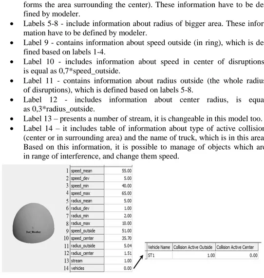
To model break in weather authors created own object with special labels and some assigned intelligence to model a particular interference (Fig.3). Each bad weather condition has been mapped on a single object named Bad_Weather. Authors created this object with using TaskExecuters Object in FlexSim. They used this type because it has additional function – definition of collision and possibility to check if other objects are in this area. Extent of this disturbance is expressed by two circle. Radius of bigger circle are defined by modeler, by using normal statistical distribution (with mean, deviation, and with minimum and max-imum value of this aspect). The radius of smaller circle (center of weather change) has been set as 0,3 radius value of a bigger circle. The same situation is about a truck’s speed – speed in the area surrounding the center are exactly defined by modeler (in labels), while speed in center is converted – 0,7 speed value.
Information about random values are description in labels in object. Created Bad_Weather object has 14 labels.
Labels 1-4 - contain information about mean, deviation, minimum and maximum value of speed in bigger area of disturbance (in the ring, which
forms the area surrounding the center). These information have to be de-fined by modeler.
Labels 5-8 - include information about radius of bigger area. These infor-mation have to be defined by modeler.
Label 9 - contains information about speed outside (in ring), which is de-fined based on labels 1-4.
Label 10 - includes information about speed in center of disruptions, is equal as 0,7*speed_outside.
Label 11 - contains information about radius outside (the whole radius of disruptions), which is defined based on labels 5-8.
Label 12 - includes information about center radius, is equal as 0,3*radius_outside.
Label 13 – presents a number of stream, it is changeable in this model too. Label 14 – it includes table of information about type of active collision
(center or in surrounding area) and the name of truck, which is in this area. Based on this information, it is possible to manage of objects which are in range of interference, and change them speed.
Fig. 3 Created Bed_Weather Object.
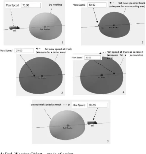
When bad weather condition occurs, area of effect is defined by normal distri-bution with parameters stored in object labels. The level of speed decrease is de-fined in the same way. Described object checks, with certain time interval, if there is another object in range. When an object (mean of transport) is detected, its travel speed is decreased to specific value, first to speed adequate to surrounding area (case 2 at Fig. 4), then to speed for center area (case 3 at Fig. 4) and then again at speed for surrounding area (case 4 at Fig. 4). When this objects leaves area, its speed is set back to original value (case 5 at Fig. 4). Checking time interval is relative small (currently 0.01 time unit). It provides, that moment when the vehi-cle has left the disturbance is quickly noticed. Figure 4 shows described situations.
Fig. 4: Bed_Weather Object – mode of action.
4.2. Description of simulation experiments
For presented simulation model with transport route four experiments (4 scenarios) were made. Each experiment was made 10 times (10 replications) to show influence of random value setting in disturbance. Experiments were made by using built-in experimenter tool in FlexSim.
In every experiments main variables in weather disturbance were changed, to show how this disruption affects to the time of realization the transport process. In present case authors do not take into account the possibility of a detour – the alternate route. The issue of seeking a new route, because of disturbances, is not the aim of this study. The main goal is show changeable time of realized transport, which depends on random value in disturbances (like radius of this dis-ruption or truck speed in area of this disdis-ruption). To show relations between
pro-cess time versus disturbances, authors made some simplifications. First: only two disruptions are considered in model. Second: acceleration and deceleration aspects are not taken into account in the model.
Table 1 Definition of simulation experiment
Experiment No Take into account the driver's working time
Definition of speed Definition of range
Mean value of speed Dev of speed Min value of speed Max value of speed Mean value of radius Dev of radius Min value of radius Max value of radius 1 yes 55 5 40 65 5 1 2 10 2 yes 60 10 40 65 10 2 2 15 3 yes 55 10 40 67 10 3 2 15 4 yes 40 15 30 55 10 5 2 15
Information about the experiments are summarized in Table 1. Important infor-mation is the fact, that the travel time from point A to point B without any disturb-ance is equal 2.38 hour.
4.3 Results of experiments
The main purpose of these experiments was present the transportation time, which depends on random value in disturbances, as speed and radius. Table 2 pre-sents results of this experiments. As we can see, the transportation time is the smallest at experiment 1, because the values in weather disturbance are the least slow down the process. The smallest speed, and the largest radius of this disrup-tions was defined at scenarios 4, which is reflected in the obtained results.
By using built-in experimenter tool in FlexSim, we can have information about interval of values of the analyzed time for the confidence interval as 90, 95 or 99%. Figure 6 presents results for 90% confidence interval. Referring to the description of model of supply system and given there question about existence of time of starting the loading , which ensures ending the delivery at defined interval , we can say- that it exists and it can be defined it by using Exper-imenter tool in FlexSim software.
Table 2 Results of simulation experiments. Source: results obtained from FlexSim model
Transportation Time [h]
Rep 1 Rep 2 Rep 3 Rep 4 Rep 5 Rep 6 Rep 7 Rep 8 Rep 9 Rep 10
Sc. 1 2,48 2,46 2,46 2,44 2,45 2,51 2,46 2,44 2,44 2,48
Sc. 2 2,61 2,52 2,65 2,50 2,57 2,60 2,47 2,48 2,52 2,46
Sc. 3 2,59 2,46 2,47 2,51 2,51 2,53 2,47 2,53 2,49 2,61
Sc. 4 2,72 2,56 2,75 2,72 2,91 2,91 2,55 2,47 2,45 2,75
5. CONCLUSION AND FURTHER INVESTIGATIONS
The presented approach to modeling a supply chain enables precision analysis of processes and impact of them to whole transport process. Thanks to using the simulation, observation and analysis of process is possible. In addition, including aspect of disturbances, a good tool to determine the time required for transport is created. Authors in detailed description present a way of modeling processes in supply chain and disturbances. In order to show the use of the described aspects, the simulation model for the sample transport routes have been created. By per-forming a number of experiments is shown a relationship between "the strength" of the interference and times of transport realization.
Obviously, there is an opportunity for further development of the proposed work: modelling next disturbances in described way (with combining ABS and DES approach). And check relation between them and time of realization the transport task. Creating library with disturbances, fast building of simulation model will be possible. Next step is "play" with simulation model and definition of time of analyzed process, with using build-in experimenter tool.
ACKNOWLEDGEMENTS
Presented research are carried out under the LOGOS project (Model of coordi-nation of virtual supply chains meeting the requirements of corporate social re-sponsibility) under grant agreement number PBS1/B9/17/2013.
REFERENCES
Balbo, F.& Pinson, S., (2005), Dynamic modeling of a disturbance in a multi-agent system for traffic regulation, Decision Support System 41, pp. 131-146.
Bocewicz, G., Nielsen, P., Banaszak, Z. & Dang, Q.V., (2013), Multimodal Processes Cyclic States Scheduling. In: Corchado, J.M., Bajo, J., Kozlak, J., Pawlewski, P., Molina, J.M.,
Julian, V., Silveira, R.A., Unland, R., Girox, S. (eds.) Higlights on Practical Applications of Agents and Multi-Agent Systems, pp. 73-85, Springer, Heidelberg.
Caddy, I.N. & Helou, M.M., (2007), Supply chains and their management: Application of general systems theory, Journal of Retailing and Consumer Services 14, pp.319-327. Cassandras, C.G. & Lafortune, S., (2008), Introduction to Discrete Event Systems Second
Edition, Springer, ISBN-13: 978-0-387-33332-8, pp. 557-615.
Chen, S., Peng, H., Liu, S. & Yang, Y. 2009. A Multimodal Hierarchical-based Assignment Model for Integrated Transportation Networks, Journal of Transportation Systems Engineering and Information Technology, Vol.9, Issue 6, pp. 130-135.
Gheorghe, A., Birchmeier, J. & Kröger W., (2004), Advanced Spatial Modelling for Risk Analysis of Transportation Dangerous Goods, In: Spitzer, C. et al. (eds.), Probabilistic Safety Assessment and Management, Springer, pp. 2499-2504.
offa, P. & Pawlewski, P., (2014a), Agent Based Approach for Modeling Disturbances in Supply Chain, In Corchado, J.M., Bajo, J., and Other, (ed.), Highlights of Practical Applications of Heterogeneous Multi-Agent Systems, Communications in Computer and Information Science, pp. 144-155.Springer, Heidelberg.
Hoffa P. & Pawlewski P., (2014b), Models of Organizing Transport Tasks Including Possible Disturbances and Impact of Them on the Sustainability of the Supply Chain, Pawlewski P, Greenwood A. (Eds.), Process Simulation and Optimization in Sustainable Logistics and Manufacturing, Eco Production. Environmental Issues in Logistics and Manufacturing, Springer Cham Heidelberg New York Dordrecht London, pp. 141-151. Kim, S.-H. & Robertazzi, T.G., (2006), Modeling Mobile Agent Behavior, Computers and
Mathematics with Applications 51, pp. 951-966.
Macal, C.M., North & M.J. 2013 Introductory tutorial: Agent-Based Modeling and Simulation, Winter Simulation Conference, pp. 362-376.
Marseguerra, M., Zio, E. & Bianchi, M., (2003), A fuzzy model for the estimate of the accident rate in road transport of hazardous materials, In: Bedford & van Gelder (eds),Safety and Reliability, Swets & Zeitlinger, Lisse, pp. 1085-1092.
Skorupski, J., (2011), Sieci Petriego jako narzędzie do modelowania procesów ruchowych w transporcie, Prace Naukowe Politechniki Warszawskiej, Transport, z.78, s. 69-84. Wieland, A. & Wallenburg, C.M., (2011), Supply-Chain-Management in stürmischen
Zeiten. Berlin.
Wilhelm, T. & Hollunder, J., (2007), Information theoretic description of networks, Physica A, Vol.385, Issue 1, pp. 385-396.
http://www.anylogic.com/agent-based-modeling, access date: 01.2014 https://www.flexsim.com/, access date: 01.015
http://isap.sejm.gov.pl/, access date: 01.2015
http://www.llamasoft.com/supply-chain-simulation-software.html, access date: 03.2015 http://www.traxelektronik.pl/pogoda/lokalizacja.php?RejID=8&B=1366&H=728, access
date: 03.2015
BIOGRAPHICAL NOTES
Patrycja Hoffa-Dąbrowska is PhD student at the Faculty of Engineering Man-agement at Poznan University of Technology. Her research interests include logis-tics, IT application for logislogis-tics, process modeling, simulation and optimization.
Paweł Pawlewski is professor at the Faculty of Engineering Management at Poz-nan University of Technology. His research interests include organization of manu-facturing systems, monitoring of operations management, reengineering and IT application for logistics, process modeling, simulation and optimization. He is au-thor or co-auau-thor over 120 manuscripts including books, journals and conference proceedings. He is managing director of SOCILAPP Simulation and Optimization Center in Logistics and Production Processes.